Potential Due to an Electric Dipole

An electric dipole is two equal and opposite charges, +q and −q, separated by a small distance 2a (or 2l). Its dipole moment is p = q × 2a, directed from −q to +q. Since potential is a scalar quantity, the potential due to a dipole at any point is simply the algebraic sum of the potentials due to each charge — no vector addition needed, unlike the electric field.

The potential at a general point P (distance r, angle θ from the dipole axis) directly, then derives axial and equatorial cases as special results.

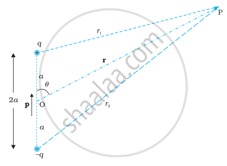
Origin is taken at the dipole center. By the superposition principle:

• Axial point (θ = 0° or 180°): V = \[\pm\frac{1}{4\pi\varepsilon_0}\frac{p}{r^2}\]​ (+ for θ = 0°, − for θ = 180°)
• Equatorial point (θ = 90°): V = 0

Key contrasts with a single point charge

• Dipole potential depends on both r and θ (angle between r and p), not just r; it is axially symmetric about p.
• Dipole potential falls off as 1/r² at large distances, not as 1/r like a single point charge.

This approach builds up the result by solving axial, equatorial, and general points separately, using perpendicular-distance geometry with half-length l.

Case 1: Potential on the Axial Line

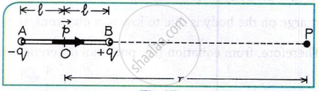
Let P lie on the line through both charges, at distance r from the dipole's center, with half-length l.

• Distance from +q to P: (r − l)
• Distance from −q to P: (r + l)

Adding potentials algebraically:

Simplifying, with dipole moment p = 2ql:

For r >> l, the l² term is negligible:

Point P lies on the perpendicular bisector of the dipole, equidistant from +q and −q (BP = AP).

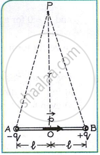
The two potential contributions are equal in magnitude but opposite in sign, so they cancel:

Key insight: Even though the potential is zero here, the electric field is not zero — no work is done moving a charge along this line, but a force still acts on it.

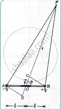
For point P at distance r and angle θ from the dipole axis (r >> l), using perpendiculars AD and BC onto OP:

• BP ≈ r − l cos θ
• AP ≈ r + l cos θ

Since r >> l, the l² cos²θ term is negligible:

Vector form:

This matches Method 1 exactly — confirming both derivations converge to the same result. Setting θ = 0° recovers the axial case; θ = 90° gives the equatorial case (V = 0).

Given: q = 3 × 10^-9 C, separation 2l = 10 cm (l = 0.05 m), r = 20 cm (0.2 m), k = 9 × 10⁹ N·m²/C²

Formula: V = kp / (r² − l²), where p = q × 2l = 3 × 10^-10 C·m

Solution: V = \[\frac{9\times10^9\times3\times10^{-10}}{(0.2)^2-(0.05)^2}=\frac{2.7}{0.0375}\]

Answer: V = 72 volts

A water molecule (H₂O) behaves like a natural electric dipole — its oxygen and hydrogen atoms carry small opposite charges separated by a tiny distance. The same "potential depends on direction" behavior explains why water is such an effective solvent at the molecular level.