Determination of Price and Equilibrium Under Monopoly - Total Revenue and Total Cost Approach

A monopolist wants to choose that level of output where profit is highest.
Profit is the difference between Total Revenue (TR) and Total Cost (TC), so:
$\pi =\; TR\; -\; TC$

In the TR–TC approach, the monopolist looks for the output level at which this difference (TR − TC) is maximum.​

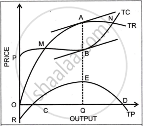
1. TR curve

• TR starts from the origin, because when output is zero, total revenue is also zero.
• As output increases, TR increases, typically at a decreasing rate for a monopolist.​

2. TC curve

• The TC curve starts from a positive point on the vertical axis (point P), because even if production is zero, the firm must pay fixed costs.
• As output increases, TC rises, generally at an increasing rate due to rising marginal costs.​

3. TP (Total Profit) curve

• TP = TR − TC at each output level.
• At very low output, TC is greater than TR, so TP is negative; the TP curve starts below the horizontal axis (point R), showing loss.
• As output increases, TR starts to overtake TC, and TP rises; the TP curve slopes upward until it reaches a maximum at point E.
• At point E, the vertical distance between TR and TC is greatest, so profit is maximum; the corresponding output is the equilibrium output of the monopolist.​

4. Break-even point (point M)

• At point M, TR = TC, so profit is zero.
• This is called the break-even point, and it separates the loss region (to the left of M, where TC > TR) from the profit region (to the right of M, where TR > TC).​

For very low output:

• TR is low but TC is relatively high due to fixed costs.
• TR < TC → firm incurs loss; TP curve lies below the axis.

At some higher output (point M):

• TR = TC → zero profit; break-even situation.

Between break-even and the profit-maximising output:

• TR > TC → firm earns positive profit; TP curve slopes upwards.

At the equilibrium output (corresponding to point E on the TP curve):

• TR − TC is maximum → profit is maximum and the monopolist is in equilibrium.

Beyond equilibrium output:

• If output increases further, TC rises faster than TR, and the difference TR − TC starts to fall; profit falls.​

In practice, the monopolist may not know in advance which output gives maximum profit.
The firm can:

• Choose different possible prices and calculate the corresponding quantity demanded, TR, TC, and profit;
• Compare the profits at each output level;
• Stop at the output where profit is highest.

This practical process of trying different price–output combinations and selecting the best one is called the trial-and-error approach to monopoly equilibrium.​

• The profit of a monopolist is the difference between TR and TC, i.e., π = TR − TC.​
• Under the TR–TC approach, the monopolist chooses that output where the difference TR − TC is maximum.
• The TR curve usually starts from the origin, while the TC curve starts above the origin due to fixed costs.​
• The break-even point is where TR = TC and profit is zero.
• The equilibrium output of the monopolist is found where the vertical distance between TR and TC is greatest, which corresponds to the highest point on the TP curve (point E).
• The process is called trial-and-error because the firm may test different price–output combinations to discover where profit is highest.