Topics
National Income and Related Aggregates
- Macroeconomics Vs Microeconomics
- Representative Goods and Sectors
- Macroeconomic Agents and Government Role
- Emergence of Macroeconomics
- Context of the Present Book of Macroeconomics
- Meaning of Economic Wealth and Final Goods
- Stocks, Flows, and Depreciation
- Capital Formation, Trade-off & Circular Flow of Income
- Circular Flow of Income and Methods of Calculating National Income
- Output Method/Product Method
- Expenditure Method
- Income Method
- Factor Cost, Basic Prices and Market Prices
- Some Macroeconomic Identities
- National Disposable Income
- Private Income
- National Income Aggregates
- Real GDP and Nominal GDP
- GDP and Welfare
Introductory Macroeconomics
Introduction
- A Simple Economy
- Central Problems of an Economy
- Concepts of Production Possibility Frontier
- Organisation of Economic Activities
- Positive and Normative Economics
- Macroeconomics Vs Microeconomics
Development Experience (1947-90) and Economic Reforms since 1991
- India's Economy Before Independence
- Low Level of Economic Development Under the Colonial Rule
- Agricultural Sector in India
- Industrial Sector
- Foreign Trade of India
- Demographic Condition
- Occupational Structure
- Infrastructure
- Post-Independence Economic Systems and Planning
- Five Year Plans (FYP)
- Agriculture
- Industry and Trade
- Trade Policy: Import Substitution
- The 1991 Economic Crisis and Reforms
- Background of the New Economic Policy
- Liberalisation
- Privatisation
- Globalisation
- World Trade Organisation (WTO)
- Impact of the Economic Reforms
Current Challenges Facing Indian Economy
- Concept of Human Capital
- Sources of Human Capital
- Human Capital and Economic Growth
- Human Capital and Human Development
- State of Human Capital Formation in India
- Growth of Education Sector in India
- Challenges and Future Prospects in Education
- Rural Development in India
- Credit and Marketing in Rural Areas
- Agricultural Market System
- Diversification into Productive Activities
- Sustainable Development and Organic Farming
- The Nature and Importance of Work in Society
- Workers and Employment
- Participation of People in Employment
- Self-employed and Hired Workers
- Employment in Firms, Factories and Offices
- Growth and Changing Structure of Employment
- Informalisation of Indian Workforce
- Concept of Unemployment
- Government and Employment Generation
- Environment and Sustainable Development in India
- State of India’s Environment
- Concept of Sustainable Development
- Strategies for Sustainable Development
Money and Banking
- Concept of Money
- Functions of Money
- Demand for Money and Supply of Money
- Money Creation by Banking System
- Limits to Credit Creation and Money Multiplier
- Policy Tools To Control Money Supply
- Demand and Supply for Money : A Detailed Discussion
- The Transaction Motive
- The Speculative Motive
- Various Measures of Supply of Money
- Narrow and Broad Money
- Demonetisation
Theory of Consumer Behaviour
- Consumer Behaviour: The Problem of Choice
- Basic Concepts of Microeconomics > Utility
- Cardinal Approach (Utility Analysis)
- Derivation of Demand Curve in the Case of a Single Commodity
- Ordinal Utility Analysis/Indifference Curve Analysis
Indian Economic Development
Determination of Income and Employment
- Aggregate Demand and Its Components
- Consumption
- Investment
- Determination of Income in Two-sector Model
- Determination of Equilibrium Income in the Short Run
- Macroeconomic Equilibrium with Price Level Fixed
- Effect of an Autonomous Change in Aggregate Demand on Income and Output
- The Multiplier Mechanism
- Paradox of Thrift
- Equilibrium Output and Employment
Development Experience of India – a Comparison with Neighbours
Introductory Microeconomics
Production and Costs
- Production Function
- Basics of Production Theory
- Variation of Output in the Short-Run Returns to a Factor
- Relation Between Total, Average and Marginal Product
- Law of Variable Proportions
- Average and Marginal Physical Products
- Changes in Production
- Cost - Fixed Cost
- Cost -variable Cost
- Behaviour of Cost in the Short - Run
- Relationship Between Average Variable Cost and Average Total Cost and Marginal Cost
- Concept of Opportunity Cost
- Marginal Revenue
- Producer's Equilibrium
- Law of Supply
- Market Supply Schedule
- Distinguish between Stock and Supply
- Determinants of Supply
- Movements Along and Shifts in Supply Curve
- Measurement of Elasticity of Supply
- Methods of Measurement of National Income
- Cost Concepts > Marginal Cost
- The Law of Diminishing Marginal Product
- Shapes of Product Curves
- Costs in Long Run Period
- Returns to Scale
The Theory of the Firm Under Perfect Competition
- Concept of Market
- Market Equilibrium
- Determination of Market Equilibrium
- Effect of Simultaneous change in Demand and Supply on Equilibrium Price
- Perfect Competition
- Imperfect Competition
- Classification of Market Structure
- Oligopoly
- Market Forms - Perfect Oligopoly
- Market Forms - Imperfect Oligopoly
- Equilibrium Price
- Applications of Tools of Demand and Supply Price Control
- Price Ceiling
- Price Floor
- Revenue Concepts
- Profit Maximisation Objective
- Determinants of a Firm’s Supply Curve
- Market Supply Schedule
- Price Elasticity of Supply
Government Budget and the Economy
Market Equilibrium
- Simple Monopoly in the Commodity Market
- Other Non - Perfectly Competitive Markets
Balance of Payments
- Open Economy and Its Linkages
- Concept of Balance of Payments
- Current Account
- Capital Account
- Balance of Payments Surplus and Deficit
- Foreign Exchange Market
- Foreign Exchange Rate
- Determination of the Exchange Rate
- Merits and Demerits of Flexible and Fixed Exchange Rate Systems
- Managed Floating Exchange Rate System
- Introduction
- Definition: Long Run
- Definition: Long Run Total Cost
- Long Run Total Cost
- Definition: Long Run Average Cost
- Long Run Average Cost
- Names for LAC
- Relationship: LAC and SAC
- Definition: Long Run Marginal Cost
- Long Run Marginal Cost
- Relation Between LMC and LAC
- Key Points: Costs in Long Run Period
CISCE: Class 12
Introduction
- The long run is a period in which a firm can change all its inputs—including machines, buildings, and workers. No input is fixed; everything can be adjusted to change output.
- Example: If a bakery wants to bake more bread in the long run, it can buy new ovens, hire more staff, or move to a bigger location.
CISCE: Class 12
Definition: Long Run
- "In the long-run, all the factors of production are assumed to be variable." - Koutsoyiannis
- "It will be helpful to think of the long run situation into any one in which the firm can move." - Leftwich
CISCE: Class 12
Definition: Long Run Total Cost
"The long run total cost of production is the least possible cost of producing any given level of output when all inputs are variable." - Libhafasky
CISCE: Class 12
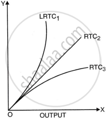
Long Run Total Cost
- LRTC: The lowest possible total cost for making any amount of goods when all inputs can vary.
- In the long run, there are no fixed costs—if nothing is produced, total cost is zero.
CISCE: Class 12
Defnition: Long Run Average Cost
"The long run average cost curve shows the lowest average cost of producing output when all inputs can be varied freely." - Robert Awh
CISCE: Class 12
Long Run Average Cost
- Formula:
\[\overline{\mathrm{LAC}=}\frac{\mathrm{LRTC}}{\text{Quantity of Output}}\] - LAC curve shows the lowest average cost per unit when all factors can be chosen.
- Analogy: Think of LAC as the “cheapest possible menu” you could pick to feed your group, if you could freely select all ingredients and cooking tools.
CISCE: Class 12
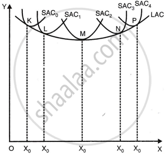
Names for LAC
- Envelope Curve: LAC surrounds all the short-run average cost (SAC) curves; it never rises above them, just touches them.
- Planning Curve: Helps firms decide which plant size is best for different output levels.
CISCE: Class 12
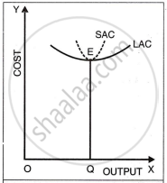
Relationship: LAC and SAC
- SAC is for a single plant; LAC is for the best of all possible plant choices.
- Both are usually U-shaped, but LAC is flatter, showing costs change less sharply in the long run.
- LAC touches only one SAC at its lowest point; for others, tangency is not at their minimum.
CISCE: Class 12
Definition: Long Run Marginal Cost
"Long-run marginal cost curve is that which shows the extra cost incurred in producing one more unit of output when all inputs can be changed." - Robert Awh
Long Run Marginal Cost
- LMC: Extra cost for making one more unit when all inputs can be changed.
- Formula:
\[\overline{\mathrm{LMC}=\frac{\Delta\mathrm{LTC}}{\Delta Q}}\]
CISCE: Class 12
Relation Between LMC and LAC
The connection between long run marginal cost (LMC) and long run average cost (LAC) works just like the short-run case:
- When LAC is falling: LMC is below LAC, and it falls faster than LAC.
- At the minimum point of LAC: LMC and LAC are equal. This is where both curves meet.
- When LAC is rising: LMC is above LAC and increases faster than LAC.
CISCE: Class 12
Key Points: Costs in Long Run Period
- In the long run, firms can change all production factors for least cost.
- LAC curve helps in selecting the best way to produce for each output.
- LMC tells us how much extra cost is needed to raise output by one unit.
- Understanding cost curves helps firms plan profitably for both present and future production.
