Propensity to Consume or Consumption Function

• The consumption function or propensity to consume shows the relationship between income (Y) and planned consumption expenditure (C) of households.
• In symbols, this relationship is written as:

C = f(Y)

This means that consumption depends on income.

• "The consumption function shows what changes can be expressed in the consumption from given changes in income." — Hansen
• "Consumption function is nothing more than a statement of the relation between consumption, expenditure and income." — R.G. Lipsey
• "It is a functional relationship indicating how consumption varies when income varies." — Dillard
• "Consumption function may be defined as a schedule showing amounts that will be spent for consumer goods and services at different income levels." — Peterson

• On a graph, income (Y) is on the horizontal axis and consumption (C) on the vertical axis.
• At any point on the consumption curve CC, APC equals the ratio of the vertical distance to the horizontal distance from the origin:
  \[APC=\frac{\text{vertical distance (C)}}{\text{horizontal distance (Y)}}\]
• Geometrically, it is the slope of the ray drawn from the origin to the point on the consumption curve.

• The slope of the consumption curve CC represents MPC.
• Between two points KK and LL on the consumption curve:
  \[MPC=\frac{\Delta C}{\Delta Y}=\frac{\text{vertical change KL}}{\text{horizontal change Y1Y2}}\]
• For a linear (straight-line) consumption function, MPC is constant at all income levels.

1. Consumption varies directly with income

• When income increases, desired consumption increases; when income falls, desired consumption falls.
• Countries with higher per capita incomes generally have higher levels of consumption.
• Symbolically:
  \[C=f(Y),\quad\mathrm{with}\frac{dC}{dY}>0\]

2. Increase in consumption is less than increase in income

• When income rises, consumption also rises, but by a smaller amount than the rise in income.
• The additional income is split between additional consumption and additional saving.
• In terms of MPC c:
  $c>0$ (consumption increases with income)
  $c<1$ (increase in consumption is less than increase in income)
  Hence:

0 < c < 1

In this chapter, a linear consumption function is assumed:

C = a + cY

Where:

• C: aggregate consumption
• Y: income
• a: autonomous consumption (positive constant) – minimum consumption even when income is zero.
• c: marginal propensity to consume (MPC) – constant slope of the consumption line.

Interpretation:

• Autonomous consumption (a): part of consumption independent of current income (basic needs financed by borrowing/dissaving).
• Induced consumption (cY): part of consumption that depends on income; it increases when income increases.
• For this linear function, MPC = cc is constant. In more general, non-linear cases, MPC may fall as income rises (people consume a smaller fraction of each additional rupee of income).

• Psychological Nature: Based on personal tastes/habits (e.g., festival shopping urge). Stays steady short-term.
• Links to Income/Jobs: Higher PTC → more spending → business growth → jobs (e.g., Diwali sales boom).
• Unequal Across Groups: Poor spend nearly all (100% PTC) on basics; rich save more (e.g., slum family vs. high-rise owner).
• Short Run: Consumption rises slower than income; PTC falls as Y grows. (See Table below.)
• Long Run: PTC stable; no "must-spend" base—full income drives spending.

Insight: At low income, borrow to eat. Beyond ₹550, extra income saves—consumption plateaus.

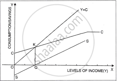
Diagram Description 
X-axis: Income; Y-axis: Consumption/Savings. 45° line = C=Y. CC curve (upward, below 45°) shows rising but slower C. SS curve starts negative (borrowing), crosses zero at breakeven. Point K: Y=C (no savings).
Real-Life Example: Mumbai street vendor spends 90% on stock/food (high PTC); banker saves 60% for flat loan (low PTC).