Propensity to Save

A saving function shows the relationship between the level of saving and the level of income.
In Keynesian economics, saving is taken as a function of income, just like consumption.

Symbolically:
S = f(Y)

• S = saving
• Y = income

In a simple two-sector economy (only households and firms), the part of income that is not spent on consumption is saved.

Algebraically:
$S=Y-C$

• C = consumption expenditure

This means:

• Every unit of income is either consumed or saved.
• There is no third use of income in this simplified model.

\[\mathrm{MPS}=\frac{\Delta S}{\Delta Y}\]

Where:

• ΔS = change in saving
• ΔY = change in income

Average Propensities: APC + APS = 1
Why? From Y = C + S, divide by Y: $YC+YS=1$.
Example: APC = 0.9, then APS = 0.1 (or vice versa).

Marginal Propensities: MPC + MPS = 1
Why? Extra income ΔY = ΔC + ΔS, divide by ΔY: ΔCΔY+ΔSΔY=1ΔYΔC+ΔYΔS=1.
Example: MPC = 0.8, then MPS = 0.2.

Quick Formulas: APC = 1 - APS; MPS = 1 - MPC.

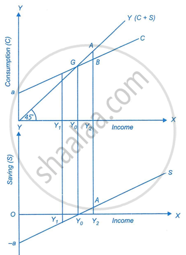
Saving curve (S) comes straight from consumption curve (C) using the 45° income line (Y = C + S).
Key Insight: Vertical gap between 45° line and C-curve = saving amount.

Step-by-Step:

1. Plot C-curve (starts at 'a' >0, slopes <45°).
2. Draw 45° line from origin (all income points).
3. S = distance between them (negative left, zero at intersection, positive right).

Visual Description:

• Upper panel: C below 45° line right of OY₀ (saving positive).
• Lower panel: S-line mirrors gaps—dissaving (OY₁), zero (OY₀), saving (OY₂).
  Gap widens rightward as income rises.

Analogy: 45° line is your full paycheck envelope; C is what you spend—remainder (gap) is pocketed.