Topics
Microeconomic Theory
Microeconomics and Macroeconomics: Introduction
Theory of Income and Employment
Demand and Law of Demand
- Role of Demand and Supply in Economics
- Paul A. Samuelson: Father of Modern Economics
- Concept of Demand
- Types of Demand
- Determinants of Demand
- Demand Function
- Law of Demand
- Demand Schedule
- Individual Demand Schedule
- Market Demand Schedule
- Demand Curve
- Individual Demand Curve
- Market Demand Curve
- Reasons for the Downward Slope of the Demand Curve
- Importance of the Law of Demand
- Exceptions to the Law of Demand
- Movement along the Demand Curve and Shift of the Demand Curve
- Change in Quantity Demanded: Movement along the Demand Curve
- Change in Demand – Shift in Demand Curve
- Difference Between Extension and Increase in Demand
- Difference Between Contraction and Decrease in Demand
Theory of Consumer Behaviour: Marginal Utility and Indifference Curve Analysis
- Basic Concepts of Microeconomics > Utility
- Cardinal Approach (Utility Analysis)
- Total Utility and Marginal Utility
- Relationship Between Total Utility and Marginal Utility
- Approaches to Consumer Behaviour
- Law of Diminishing Marginal Utility
- Alfred Marshall: Key Contributor to Economics
- Consumer's Equilibrium through Cardinal Utility Approach
- Law of Equi-Marginal Utility
- Importance and Limitations of law of Equi-Marginal Utility
- Ordinal Utility Analysis/Indifference Curve Analysis
- Marginal Rate of Substitution (MRS)
- Relationship Between Marginal Rate of Substitution and Marginal Utility
- Properties of Indifference Curves
- Price Line or Budget Line
- Consumer's Equilibrium through Indifference Curve Approach
Money and Banking
Elasticity of Demand
- Concept of Elasticity of Demand
- Types of Elasticity of Demand > Price Elasticity
- Methods of Measuring Price Elasticity of Demand
- Percentage or Proportionate Method
- Total Expenditure Method
- Point Method (Geometric Method)
- Arc Elasticity of Demand
- Revenue Method
- Numerical Problems of Price Elasticity of Demand
- Factors Affecting Price Elasticity of Demand
- Importance of Elasticity of Demand
- Types of Elasticity of Demand > Income Elasticity
- Types of Elasticity of Demand > Cross Elasticity
Balance of Payment and Exchange Rate
Supply: Law of Supply and Price Elasticity of Supply
- Concept of Supply
- Determinants of Supply
- Law of Supply
- Movements Along and Shifts in Supply Curve
- Elasticity of Supply
- Price Elasticity of Supply
- Categories (Degrees) of Elasticity of Supply
- Measurement of Elasticity of Supply > Percentage Method
- Measurement of Elasticity of Supply > Geometric or Point Method
- Determinants of Elasticity of Supply
Public Finance
Market Mechanism: Equilibrium Price and Quantity in a Competitive Market
- Basic Concepts of Equilibrium and Equilibrium Price
- Equilibrium Price and Quantity in a Competitive Market
- Effects of Changes (Shifts) in Demand on Equilibrium Price and Equilibrium Quantity
- Effects of Changes (Shifts) in Supply on Equilibrium Price and Equilibrium Quantity
- Effects of Simultaneous Changes (Shifts) in Demand and Supply
- Some Special Cases of Equilibrium
- Applications of Tools of Demand and Supply Price Control
- Mаximum Price Legislation or Price Ceiling and Rationing
- Minimum Price Legislation or Floor Price
National Income
Laws of Returns: Returns to a Factor and Returns to Scale
- Basics of Production Theory
- Products
- Factors of Production
- Production Function
- Types of Production Functions
- Basic Product Concepts
- Relationship between Average Product (AP) and Marginal Product (MP)
- Relationship between Total Product (TP) and Marginal Product (MP)
- Law of Variable Proportions
- Three Stages of Production
- Stages of Operation and the Decision to Produce
- Variation of Output in the Short-Run Returns to a Factor
- Changes in Production
- Explanation of the Law of Variable Proportions
- Variation of Output in the Long Run - Returns to Scale
- Law of Variable Proportions and Returns to Scale Compared
- Scale of Production and Concept of Indivisibility
- Economies of Scale
- Diseconomies of Scale
- Significance of Economies of Scale
Cost and Revenue Analysis
- Cost of Production
- Theories of Costs: Traditional Theory of Costs/Short Run Cost Curves
- Cost Concepts > Total Costs
- Cost Concepts > Average Cost
- Cost Concepts > Marginal Cost
- Costs in Long Run Period
- Difference Between Short - Run & Long Run Costs
- Behaviour of Cost in the Short - Run
- Relationship between Average and Marginal Cost
- Long-Run Cost Curves
- Revenue Concepts
- Types of Revenue
- Relation Between Total, Average and Marginal Revenue
- Relationship between Total, Average and Marginal Revenues under Perfect Competition
- Relationship between Total, Average and Marginal Revenue under Imperfect Competition
- Relationship Between (Mutual Determination) AR, MR, and Elasticity of Demand
- Comparative Study of Revenue Curves under Different Markets
- Significance of Revenue Curve
Forms of Market
- Concept of Market
- Market Structure
- Classification of Market Structure
- Perfect Competition
- Monopoly
- Monopolistic Competition
- Oligopoly
- Duopoly
- Bilateral Monopoly
- Concept of Monopsony
- Other Forms of Market
- Factors Determining Market / Extent of Market
- Demand Curves of Firms under Different Market Forms
- Comparison between different forms of market
Producer's Equilibrium
Equilibrium of Firm and Industry Under Perfect Competition
- Concept of Equilibrium in Economics
- Firm's Equilibrium
- Producer's (Firm's) Equilibrium: Total Revenue and Total Cost Approach
- Producer's (Firm's) Equilibrium: Marginal Revenue and Marginal Cost Approach
- Determination of Short Run Equilibrium of a Firm
- Firm is a Price Taker, Not a Price Maker
- Determination of Long Run Equilibrium of a Firm
- Equilibrium of Industry
- Difference Between Firm and Industry's Equilibrium
Producer's Equilibrium Under Perfect Competition
Determination of Equilibrium Price and Output Under Perfect Competition
- Perfect Competition
- Price Determination Under Perfect Competition
- Changes in Equilibrium
- Effects of Changes (Shifts) in Demand on Equilibrium Price and Equilibrium Quantity
- Time Element in the Theory of Price Determination
- Determination of Equilibrium Prices
- Normal Price and Law of Returns
- Comparison between Market Price and Normal Price
- Practical Applications of Tools of Demand and Supply Analysis
- Determination of Short Run Equilibrium of a Firm
- Determination of Long Run Equilibrium of a Firm
Price Output Determination Under Monopoly
Price Output Determination Under Monopolistic Competition and Oligopoly
- Imperfect Competition
- Monopolistic Competition
- Equilibrium Price and Output under Monopolistic Competition
- Group Equilibrium in Monopolistic Competition
- Product Differentiation
- Selling Costs
- Oligopoly
- Price and Output Determination under Oligopoly
- Price Rigidity-Sweezy's Kinky Demand Curve Model or Equilibrium under Independent Action
- Cournot's Model
- Collusive Oligopoly
- Mergers
Theory of Income and Employment
- Basic Model of Income Determination
- Aggregate Demand and Its Components
- Propensity to Consume or Consumption Function
- Propensity to Save
- Investment Expenditure
- Determination of Equilibrium Income and Output
- Saving-investment Approach
- Investment Multiplier and Its Mechanism
- Solved Problems on Consumption and Income
- The Concept of Full Employment
- Important Terms of Employment and Unemployment
- Excess Demand
- Deficient Demand
Basic Concepts of Macro Economics
Aggregate Demand and Supply-Determinants of Equilibrium
Consumption Function (Propensity to Consume)
- Propensity to Consume or Consumption Function
- Kinds or Technical Attributes of Propensity to Consume > Average Propensity to Consume
- Kinds or Technical Attributes of Propensity to Consume > Marginal Propensity to Consume
- Propensity to Save
- Determinants of Propensity to Consume
- Psychological Law of Propensity to Consume
- Measures to Raise Propensity to Consume
Concept of Investments-Types and Determinants
Multiplier - I : Static and Dynamic
Full Employment and Voluntary Unemployment
Problems of Deficient Demand and Excess Demand
Measures to Correct Deficient and Excess Demand
Money: Meaning and Functions
Banks: Commercial Bank and Central Bank
- Concept of Bank
- Types of Bank
- Commercial Banks
- Banking > Functions of Commercial Bank
- Credit Creation by Commercial Banks
- Role of Commercial Banks in an Economy
- Central Bank
- Comparison Between Central Bank and Commercial Banks
- Central Bank as a Controller of Credit
- Methods of Credit Control
- Quantitative Methods
- Qualitative (Or Selective) Methods
Balance of Payment and Exchange Rate
- Concept of Balance of Payments
- Features of Balance of Payment
- Balance of Trade and Balance of Payments- Comparison
- Structure of Balance of Payment
- Methods to Measure Balance of Payments
- Components of Balance of Payments
- Current Account Transactions
- Capital Account Transactions
- Balance of Payments Always Balances
- Categories of Balance of Payments
- Balance of Payments Disequilibrium
- Measures to Correct Disequilibrium in the Balance of Payments
- Foreign Exchange Rate
- Exchange Rate
- Types of Foreign Exchange Rate
- Fixed Rate of Exchange
- Flexible Rate of Exchange
- Managed Floating Exchange Rate System
- Determination of Equilibrium Rate of Exchange
- Factors or Determinants of Foreign Exchange Rate
- Concepts of Depreciation, Appreciation, Devaluation and Revaluation
- Determination of Exchange Rate in a Free Market
Fiscal Policy
- Structure of Public Finance > Fiscal Policy
- Public Finance
- Instruments of Fiscal Policy
- Objectives of Fiscal Policy
- Miscellaneous Objectives of Fiscal Policy
- Fiscal Measures for Stabilisation
- Methods of Fiscal Policy in Developing Countries
- Limitations of Fiscal Policy
- Structure of Public Finance > Public Revenue
- Instruments of Fiscal Policy - Taxation
- Types of Taxes
- Tax Reforms in India
- Proportional, Progressive and Regressive Taxes
- Structure of Public Finance > Public Expenditure
- Importance of Public Expenditure
- Structure of Public Finance > Public Debt
- Reasons for Borrowing by the Government
- Public Debt - Redemption
- Deficit Financing
- Fiscal Policy in Action
Government Budget
- Budget
- Types of Budget
- Government Budget
- Need and Importance of Government Budget
- Types of Government Budget in India
- Components (Structure) of the Government Budget
- Modern Classification of Budget
- Classification of Budget Receipts
- Balanced Budget Vs Unbalanced Budget
- Zero-Base Budgeting (ZBB)
- Zero-Base Budgeting in India
- Concepts Related to Budget Deficits
- Constituents of budget /Structure of the budget
- Structure of Public Finance > Public Expenditure
- Revenue Expenditure and Capital Expenditure
- Developmental and Non-developmental Expenditure
- Tax Revenue
- Public Revenue > Non-tax Revenue
- Capital Receipts
- Objectives of Budget
- Significance of Budget
- Types of budget deficit
- Budgetary Procedure
National Income and Circular Flow of Income
- Concept of National Income
- Domestic Income
- National Income Aggregates
- Significance or Importance of National Income
- Circular Flow of Income
- Circular Flow in a Closed Economy
- Circular flow and the Equality between Production, Income and Expenditure
- Circular Flow in a Open Economy
- Economic Sectors of an Economy
- Two-Sector Model without Savings and Investment
- Two-Sector Model with Savings and Investment
- Three-Sector Model of Circular Flow of Income
- Four-Sector Model of Circular Flow of Income
- Significance or Importance of Circular Flow of Income
National Income Aggregates
- Key Relationships Among National Income Aggregates
- National Income Aggregates
- Gross Domestic Product at Market Price
- Gross National Product at Market Price
- Constituents of GNP
- Net Domestic Product at Market Price
- Difference between Net Domestic and Net National Product at Market Price
- Net National Product (NNP)
- Difference between Net National and Gross National Product at Market Price
- Net National Income or Product at Factor Cost
- Net Domestic Product or Income at Factor Cost
- Difference between Net Domestic Product at Factor Cost and Net Domestic Product at Market Price
- Gross Domestic Product or Income at Factor Cost
- Gross National Product at Factor Cost
- Factor Income from Net Domestic Product accuring to Private Sector
- Private Income
- Difference between National and Private Income
- Personal Income of National Income
- Difference between Private and Personal Income
- Disposable Income Aggregates
- Per Capita Income
- Real Income
- Interrelationship among National Income Aggregates
- Real GDP and Nominal GDP
- Gross Domestic Product (National Income) and Economic Welfare
Methods of Measuring National Income
- Concept of National Income
- Methods of Measurement of National Income
- Net Product or Value Added Method
- Precautions in the Estimation of National Income by Value-added Method
- Difficulties in the Estimation of National Income by Value-added Method
- Income Method
- Expenditure Method
- Precautions in the Estimation of National Income by Expenditure Method
- Alternative Methods of National Income Estimation
- Reconciling The Three Methods Of Estimating National Income
- Components of Net National Product at Factor Cost in its Three Phases
- Transactions Included in National Income
- The Identity of Output, Income and Expenditure
- Significance of three Methods
- Transactions not Included in National Income
- Numericals on Income, Product and Expenditure Method
National Income and Economic Welfare
- Welfare Economics
- Definitions of Welfare Economics
- Factors Determining the Size of National Income
- National Income and National Welfare
- Relation between Economic Welfare and National Income
- National Income as a Measure of Economic Welfare
- Causes of Slow Growth of National Income
- Suggestions for Increasing National Income
- Introduction
- Numerical illustration of TVC and MC
- Diagram: TVC as area under MC
- U-Shaped Nature of the Marginal Cost Curve
- Perfect competition and revenue curves
- Conditions of producer’s equilibrium
- Key Points: Producer's Equilibrium under Perfect Competition
Introduction
- Producer’s equilibrium is the level of output at which the firm maximises its profit.
- Under perfect competition, the firm is a price taker; its price, average revenue (AR) and marginal revenue (MR) are equal and constant.
- The firm’s equilibrium output is where MR = MC and MC is rising.
- Total variable cost (TVC) is the sum of marginal costs (MC) of all units produced.
Numerical illustration of TVC and MC
Consider the following (illustrative) cost schedule:
| Output (units) | TVC (₹) | MC (₹) = TVCₙ − TVCₙ₋₁ |
|---|---|---|
| 0 | 0 | – |
| 1 | 20 | 20 − 0 = 20 |
| 2 | 40 | 40 − 20 = 20 |
| 3 | 55 | 55 − 40 = 15 |
| 4 | 80 | 80 − 55 = 25 |
- TVC at 4 units of output = 80.
- Sum of MC for 1 to 4 units = 20 + 20 + 15 + 25 = 80.
- Therefore:
TVC = ∑MC
(from the first unit up to the given level of output).
Diagram: TVC as area under MC
- X-axis: Output (O to L).
- Y-axis: Cost.
- Draw a U-shaped MC curve:
(i) Initially downward sloping (MC falling).
(ii) Then bottoming out (MC at minimum).
(iii) Finally, upward sloping (MC rising). - Shade the area under the MC curve from O to L units of output.
- Label the area OLSK as TVC.
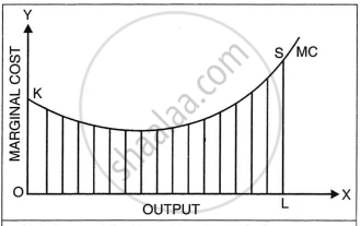
Key point:
-
TVC is equal to the sum of marginal costs of all units produced, which is represented by the area under the MC curve between O and L.
U-Shaped Nature of the Marginal Cost Curve
Due to the law of variable proportions:
- At first, when a variable factor (like labour) is increased with a fixed factor (like machinery), the firm uses resources more efficiently. Output rises more than proportionately, so marginal cost falls.
- After a certain point, too much of the variable factor with the same fixed factor leads to overcrowding, pressure on machines, and inefficiency. Output from each extra unit of input rises less and finally falls, so marginal cost rises.
Therefore, MC curve first falls, then remains roughly constant, and finally rises, giving it a U-shape.
This shape results from production technology and is common in all market forms (perfect competition, monopoly, etc.).
Perfect competition and revenue curves
Under perfect competition:
- A firm is a price taker. It accepts the market price determined by the industry where market demand equals market supply.
- Price (P) remains constant for the firm, whatever quantity it sells.
Therefore, for an individual firm:
P = AR = MR
and the AR and MR curves are horizontal straight lines at the level of the market price.
Conditions of producer’s equilibrium
A firm reaches equilibrium (profit is maximised) when both of these conditions are satisfied:
- First condition: MR = MC
- Second condition: MC is rising at the point of equality
Key Points: Producer's Equilibrium under Perfect Competition
- TVC is the sum of marginal costs of all units produced; graphically, it is the area under the MC curve between the origin and the chosen output.
- The MC curve is U-shaped due to the law of variable proportions (initial increasing returns followed by diminishing returns).
- Under perfect competition, the firm is a price taker; hence P = AR = MR and the MR curve is horizontal.
- Producer’s equilibrium (profit-maximising output) is attained where:
MR = MC, and
MC is rising and cuts MR from below. - At this equilibrium output, the difference between total revenue and total cost (profit) is maximum, and the firm has no incentive to change its level of output.
