Topics
Electrostatics
Electric Charges and Fields
- Electric Charge
- Properties of Electric Charge
- Simple Atomic Structure
- Conductors and Insulators
- Mechanism of Charging of an Object
- Charging by Friction
- Charging by Conduction
- Charging by Induction
- Coulomb's Law (Scalar Form): Force Between Two Point-Charges
- Coulomb's Law in Vector Form
- Forces Between Multiple Charges: Superposition Principle
- Equilibrium of System of Charges
- Electric Field
- Intensity of Electric Field
- Electric Field Intensity Due to a Point-Charge
- Intensity of Electric Field due to a Continuous Charge Distribution
- Electric Lines of Force
- Electric Dipole
- Electric Field due to an Electric Dipole
- Motion of an Electric Dipole in a Uniform Electric Field
- Effect of a Uniform Electric Field on the Motion of a Charged Particle
- Equilibrium of a Charged Body in a Uniform Electric Field
- Introduction to Gauss' Theorem of Electrostatics
- Area Vector
- Flux of a Vector Field
- Gauss' Theorem
- Gaussian Surface and its Properties
- Applications of Gauss' Theorem > Electric Field due to a Point Charge
- Applications of Gauss' Theorem > Electric Field due to an Infinite Line of Charge
- Applications of Gauss' Theorem > Electric Field due to an Infinite Plane Sheet of Charge
- Applications of Gauss' Theorem > Electric Field due to Two Infinite Parallel Sheets of Charge
- Applications of Gauss' Theorem > Electric Field Intensity Just Outside a Charged Conductor
- Applications of Gauss' Theorem > Electric Field due to a Uniformly Charged Thin Spherical Shell
- Applications of Gauss' Theorem > Electric Field due to a Uniformly Charged Sphere
Current Electricity
Electrostatic Potential, Potential Energy and Capacitance
- Introduction to Electric Potential
- Electric Potential: A Quantitative Approach
- Potential Difference
- Work Done in Moving a Charge in an Electric Field
- Acceleration of a Charged Particle Between Two Points in an Electric Field
- Electric Potential Due to a Point Charge
- Potential due to a Group of Point Charges
- Potential Gradient
- Electric Field as Gradient of Electric Potential: Relation between E and V
- Equipotential Surfaces
- Electric Potential Energy of a System of Charges
- Charged Body Between Parallel Plates
- Potential Due to an Electric Dipole
- Work Done in Rotating an Electric Dipole in an Electric Field
- Electric Potential Energy of an Electric Dipole in an Electrostatic Field
- Electrostatics of Conductors
- Free and Bound Charges
- Dielectrics
- Electric Polarisation of Dielectrics
- Capacitance of a Conductor
- Capacitance of an Isolated Spherical Conductor
- Potential Energy of a Charged Conductor
- Redistribution of Charges: Common Potential
- Introduction to a Capacitor
- The Parallel Plate Capacitor
- Expression for Capacitance of a Parallel-Plate Capacitor
- Dependence of the Capacitance of a Capacitor
- Capacitance of a Parallel-Plate Capacitor with Dielectric Slab between Plates
- Combination of Capacitors
- Energy Stored in a Charged Capacitor
- Force between the Plates of a Charged Parallel-Plate Capacitor
- Effect of Dielectric Insertion on a Capacitor: with and Without a Battery
- Variation of Electric Field and Potential Due to a Charged Sphere
Magnetic Effects of Current and Magnetism
Electric Resistance and Ohm's Law
- Introduction Tо Current Electricity
- Electric Current
- Current Density
- Electric Resistance
- Ohm's Law
- Experimental Verification of Ohm’s Law and Ohmic Resistors
- Exceptions of Ohm's Law : Non-Linear V-I Characteristics
- Mechanism of Flow of Electrons Through the Metal Conductors
- Mobility of Electrons
- Current, Drift Velocity Relation
- Derivation of Ohm's Law with Current Drift Velocity Relation
- Specific Resistance or Electrical Resistivity
- Ohm's law in Vector Form
- Colour Code of Carbon Resistors
- Combinations of Resistances
- An Important Deduction
- Electric Energy and Power
- Commercial Units of Electricity Consumption
- Introduction: D.C. Circuits and Measurements
- Electric cell
- Electromotive Force of a Cell
- Terminal Potential Difference
- Internal Resistance of a Cell
- Relation between E, V, and r
- Combinations of Cells
- Kirchhoff’s Laws
- Wheatstone Bridge
- Metre Bridge: Slide-Wire Bridge
- Potentiometer
Electromagnetic Induction and Alternating Currents
Moving Charges and Magnetism
- Introduction to Magnetic Effect of Current
- Oersted's Experiment
- Concept of Magnetic Field
- Force on a Moving Charge in a Uniform Magnetic Field
- Definition of Magnetic Field on the Basis of Magnetic Force
- Motion of Charged Particles in a Uniform Magnetic Field
- Lorentz Force
- Cyclotron
- Force on a Current-Carrying Conductor Placed in a Uniform Magnetic Field
- Magnetic Field Due to a Current-carrying Conductor: Biot-savart's Law
- Comparison of Coulomb's Law and Biot-Savart's Law
- Rules to Determine the Direction of Magnetic Field
- Applications of Biot-Savart's Law > Magnetic Field at the Axis of a Circular Current-carrying Loop
- Applications of Biot-Savart's Law > Magnetic Field Due to a Straight Current-carrying Conductor of Finite Size
- Applications of Biot-Savart's Law > Magnetic Field at the Centre of a Circular Current-carrying Loop
- Ampere’s Circuital Law
- Applications of Ampere’s Circuital Law > Magnetic Field of a Long Straight Thin Wire
- Applications of Ampere’s Circuital Law > Magnetic Field of a Long Straight Solenoid
- Applications of Ampere’s Circuital Law > Magnetic Field of a Toroidal Solenoid
- Force Between Two Parallel Current-Carrying Conductors : Definition of Ampere
- Comparison Between Electric and Magnetic Forces
- Torque on a Current-Loop in a Uniform Magnetic Field
- Atom as a Magnetic Dipole
- Moving Coil Galvanometer
- Sensitivity of a Galvanometer
- Conversion of a Galvanometer in Ammeter
- Conversion of a Galvanometer in Voltmeter
Magnetism and Matter
- Concept of Magnetism
- Current Loop as a Magnetic Dipole : Magnetic Dipole Moment of Current Loop
- Magnetic Dipole Moment of a Revolving Electron
- The Bar Magnet
- Magnetic Lines of Force
- Current-carrying Solenoid: An Electromagnetic Equivalent of a Bar-magnet
- Magnetic Field of a Magnetic Dipole (Small Bar Magnet)
- Torque on a Magnetic Dipole (Bar Magnet) in a Uniform Magnetic Field
- Potential Energy of a Magnet in a Magnetic Field
- Earth’s Magnetic Field
- Elements of the Earth's Magnetic Field > Angle of Declination
- Elements of the Earth's Magnetic Field > Angle of Dip or Magnetic Inclination
- Elements of the Earth's Magnetic Field > Horizontal Component of Earth's Magnetic Field
- Classification of Substances According to their Magnetic Behaviour
- Some Important Terms Used in Magnetism
- Properties of Dia, Para, and Ferromagnetic Substances
- Explanation of Dia, Para and Ferromagnetism on the Basis of Atomic Model of Magnetism
- Explanation of Demagnetisation by Atomic Model
- Hysteresis: Retentivity and Coercivity
- Differences in Magnetic Properties of Soft Iron and Steel
- Selection of Magnetic Materials
Electromagnetic Waves
Optics
Electromagnetic Induction
- Introduction to Electromagnetic Induction
- Magnetic Flux
- Electromagnetic Induction: Experimental Demonstration
- Faraday's Laws of Electromagnetic Induction
- Induced Current and Induced Charge
- Methods of Changing the Magnetic Flux
- Motion of a Straight Conductor in a Uniform Magnetic Field (Motional EMF)
- Motional Emf: A Conceptual Approach Based on Lenz's Law and Dynamic Flux Analysis
- Motional emf in Rotating a Conducting Rod in a Uniform Magnetic Field
- Self – Induction
- Self-Inductance of a Long Solenoid
- Energy Stored in an Inductor
- Some Examples of the Effect of Self-induced Current
- Mutual Inductance
- Mutual Inductance of Two Long Coaxial Solenoids
- Eddy Currents or Foucault Currents
Dual Nature of Radiation and Matter
Alternating Current
- Introduction to Ac and Aс Circuits
- Alternating Voltage and Current Developed in a Coil Rotating in Magnetic Field
- Some Definitions Regarding Alternating Voltage and Current
- Mean (or Average) Value of Alternating Current (or Voltage)
- Root-Mean-Square Value of Alternating Current
- Phasors and Phasor Diagrams
- Types of Ac Circuits > Circuit Containing Resistance Only
- Types of Ac Circuits > Circuit Containing Inductance Only
- Types of Ac Circuits > Circuit Containing Capacitance Only
- Types of Ac Circuits > Circuit Containing Inductance and Resistance in Series (L-r Series Circuit)
- Types of Ac Circuits > Circuit Containing Capacitance and Resistance in Series (C-R Series Circuit)
- Types of Ac Circuits > Circuit Containing Inductance and Capacitance (L-C Circuit)
- Types of Ac Circuits > Circuit Containing Inductance, Capacitance and Resistance in Series (L-C-R Series Circuit)
- Power in AC Circuit
- Wattless Current
- Half Power Points, Bandwidth and Q-Factor
- Choke Coil
- Electrical Oscillations in L-C Circuit
- Resonant Circuits
- Frequency Response of AC Circuits
- Alternating-Current Generator
- Transformers
- Utility of Alternating Current in Comparison to Direct Current
Electromagnetic Waves
- Introduction to Electromagnetic Waves
- Displacement Current
- Relation Between Conduction Current and Displacement Current
- Definition and Characteristics of Electromagnetic Waves
- Field Magnitude Relation in Free Space
- Important Characteristics of Electromagnetic Waves
- Transverse Nature of Electromagnetic Waves (Qualitative Idea)
- Transverse Nature of Electromagnetic Waves (Quantitative Analysis)
- Electromagnetic Spectrum
- Maxwell's Equation
- Energy Density in Electromagnetic Waves
- Overview: Electromagnetic Waves
Atoms and Nuclei
Ray Optics and Optical Instruments
- Ray Optics Or Geometrical Optics
- Spherical Mirrors
- Few Definitions Related to Spherical Mirrors
- Relation Between Focal Length and Radius of Curvature of a Spherical Mirror
- Rules to Trace the Image Formed by Spherical Mirrors
- Conditions of Image Formation
- Position and Nature of Image Formed by Spherical Mirrors
- Coordinate Geometry Sign Convention for Measuring Distances and Lengths
- Mirror Formula for Concave Mirror
- Mirror Formula for Convex Mirror
- Linear Magnification by Spherical Mirrors
- Uses of Spherical Mirrors
- Introduction to Refraction at a Plane Interface
- Refraction of Light
- Laws of Refraction
- The Refractive Index
- Cause of Refraction
- Physical Significance of Refractive Index
- Reversibility of Light
- Refraction through Parallel Multiple Media
- Refraction of Light Through a Rectangular Glass Block
- Real and Apparent Depths: Normal Displacement
- Critical Angle
- Total Internal Reflection
- Applications of Total Internal Reflection
- Introduction to Refraction at Curved Surfaces
- Coordinate Geometry Sign Convention for Measuring Distances and Lengths (Refraction)
- Refraction at Concave Spherical Surface
- Refraction at a Convex Spherical Surface
- Concept of Lenses
- Converging and Diverging Actions of Lenses
- Some Definitions Related to Lens
- Lens Maker's Formula
- Factors Affecting Focal Length of a Lens
- Image Formation by Thin Lenses
- Ray Diagrams for Formation of Image by a Convex Lens
- Image Formation by Lenses Made of Multiple Materials
- Ray Diagram for Formation of Image by a Concave Lens
- Linear Magnification by Spherical Lenses
- Power of a Lens
- Combined Focal Length of Two Thin Lenses in Contact
- Combination of Lenses and Mirrors
- Prism
- Refraction Through a Prism
- Specific Conditions for Emergent Ray
- Dispersion of White Light by a Prism : Angular Dispersion
- Dispersive Power of an Optical Medium
- Rainbows
- Scattering of Light-Rayleigh's Law
- Phenomena Based Upon Scattering of Light
- Introduction to Optical Instruments
- Power of Aссоmmodation of the Eye
- Visual Angle : Magnifying Power of Optical Instruments
- Magnifying Power of Microscope and Telescope in Terms of Visual Angle
- Simple Microscopе
- Compound Microscope
- Astronomical Telescope (Refracting Type)
- Reflecting Telescope
- Telescope Vs Compound Microscоре
- Resolving Power of Optical Instruments
- Overview: Reflection of Light: Spherical Mirrors
Electronic Devices
Communication Systems
Wave Optics
- Introduction to Wave Optics
- Wavefront
- Wave Nature of Light and Huygens' Principle
- Huygens Principle
- Behaviour of Plane Wavefront in Reflection and Refraction
- Reflection of a Plane Wave by a Plane Surface
- Refraction of a Plane Wave
- Optical Path
- Effect on Wavelength of Light in Going from One Medium to Another
- Interference of Light
- Principle of Superposition of Waves
- Interference of Light Waves and Young’s Experiment
- Conditions for Constructive and Destructive Interference of Light
- Some Additional Information about Interference
- Expression for Fringe Width in Young's Double-slit Experiment
- Change in Fringe Width Under Various Conditions
- No Interference by Two Independent Light-Sources : Coherent Sources
- Conditions for Sustained Interference of Light Waves
- Effect of Introducing a Thin Transparent Plate in the Path of One of the Interfering Beams
- Diffraction of Light
- Types of Diffraction
- Fraunhofer's Diffraction Due to a Single-slit
- Interference Vs Diffraction
- Overview: Wave Optics
Dual Nature of Radiation and Matter
- Understanding Dual Nature of Radiation and Matter
- Electron Emission
- Photoelectric Effect - Hertz’s Observations
- Hertz and Lenard's Observations
- Laws of Photoelectric Emission
- Planck's Photon Hypothesis: Quantisation of Radiation
- Einstein's Explanation of Photoelectric Effect: Photoelectric Equation
- Determination of Planck's Constant
- Energy and Momentum of Photon
- Particle Nature of Light: The Photon
- Wave Nature of a Particle: De-broglie's Thought
- de-Broglie Wavelength of Matter Waves
- Salient Features of Matter Waves
- de-Broglie Wavelength of Electron
- Experimental Demonstration of de-Broglie (Matter) Waves
- Overview: Dual Nature of Radiation and Matter
Atoms
- Atoms: Windows into Thе Invisible World
- Alpha-particle Scattering and Rutherford’s Nuclear Model of Atom
- Distance of Closest Approach of α-particle to the Nucleus-size of Nucleus
- Atomic Models: Historical Development
- Rutherford’s Atomic Model
- Atomic Spectra
- Bohr’s Model for Hydrogen Atom
- Bohr's Theory of Hydrogen-like Atoms: Radii of Permitted Orbits
- Discrete Energy Levels of Atom
- Explanation of the Line Spectrum and Estimation of Wavelength by Energy Transitions
- Hydrogen Spectrum
- Excitation and Ionisation Energy of Hydrogen Atom
- Uses of Rydberg Constant
- De Broglie’s Explanation of Bohr’s Second Postulate of Quantisation
- Overview: Atom, Origin of Spectra : Bohr's Theory of Hydrogen Atom
Nuclei
- Introduction to the Physics of the Nucleus
- Nuclear Force
- Atomic Masses and Composition of Nucleus
- Nuclear Size, Shape and Density
- Atomic Masses : Unified Atomic Mass Unit
- Isotopes
- Isobars
- Isotones
- Mass - Energy
- Pair-Production and Pair-Annihilation
- Mass Defect and Binding Energy
- Nuclear Reactions
- Q-value (Disintegration Energy) Or Energy of Nuclear Reaction
- Nuclear Energy and Stability: Exothermic Nuclear Reactions
- Nuclear Fission
- Chain Reaction in Nuclear Fission
- Multiplication or Reproduction Factor of a Chain Reaction
- Differences Between Radioactive Decay and Nuclear Fission
- Nuclear Reactor
- Nuclear Fusion
- Nuclear Bomb
- Chain Reaction-Controlled and Uncontrolled; Nuclear Reactor and Nuclear Bomb
- Stellar Energy Or Thermonuclear Energy
- Nuclear Holocaust
- Overview: Nuclei
Semiconductor Electronics
- Concept of Semiconductor Electronics
- Materials-Conductors, Insulators and Semiconductors
- Energy Bands in Materials
- Classification of Metals, Conductors and Semiconductors
- Electrons and Holes in Semiconductors
- Intrinsic Semiconductor
- Extrinsic Semiconductor
- Distinction Between Intrinsic and Extrinsic Semiconductors
- N-type VS P-type Semiconductors
- Electric Current in an Intrinsic Semiconductor
- Electric Conductivity and Resistivity of an Intrinsic Semiconductor
- Formation of P-N Junction
- Flow of Current Across Junction Diode: Forward and Reverse Biasings of Junction
- I-V characteristics in Forward and Reverse Biased P-N Junction Diode
- p-n Junction Diode as a Rectifier
- Special Purpose P-n Junction Diodes
- Overview: Semiconductor Electronics
Junction Diodes
Junction Transistors
Logic Gates
Communication Systems
Introduction
Just as wind flow can be visualised using streamlines, an invisible electric field can be visualised using electric lines of force. This concept converts an abstract, three-dimensional vector field into an intuitive picture that helps in solving both theoretical and numerical problems quickly.
Definition: Electric Lines of Force
Electric line of force is an imaginary curve drawn in an electric field such that the tangent at any point on it gives the direction of the electric field at that point.
- It represents the path along which a unit positive test charge would tend to move if free to do so.
- Lines are imaginary — they have no physical existence; they are a visualization tool only.
Properties of Electric Lines of Force
| Property | Explanation |
|---|---|
| Origin & termination | Start on positive charge, end on negative charge (or extend to/from infinity for a single charge) |
| Tangent rule | Tangent at any point gives direction of E at that point |
| Non-intersecting | Two field lines never cross, since E cannot have two directions at one point |
| Density ∝ field strength | Closely spaced lines = stronger field; widely spaced = weaker field |
| Conductor surface | In equilibrium, lines are normal (perpendicular) to a conductor's surface |
| Zero field inside conductor | No field lines exist inside a charged conductor in electrostatic equilibrium |
| Continuity | In charge-free space, lines are treated as continuous curves |
| No closed loops | Electrostatic field lines never form closed loops (unlike magnetic field lines) |
Electric Field Diagram Gallery
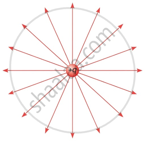
1. Isolated Positive Charge: This diagram shows the electric field originating from a single, isolated positive charge. The field lines are directed radially outward, reflecting the repulsive nature of the charge.
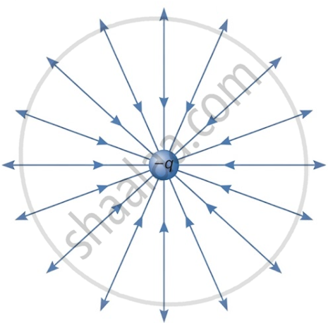
2. Isolated Negative Charge: In contrast to the positive charge, this diagram shows the electric field lines for an isolated negative charge. The lines are directed radially inward, indicating the direction a positive test charge would be pulled.
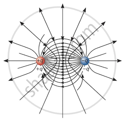
3. Electric Dipole: This diagram visualizes the field created by two equal and opposite charges. The field lines are curved, starting on the positive charge (+q) and terminating on the negative charge (−q). The field is densest in the region directly between the two charges.
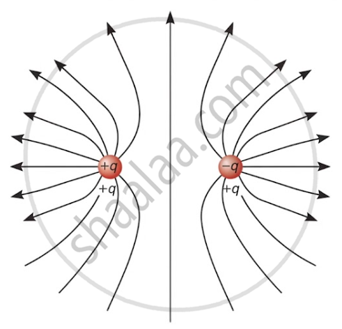
4. Two Equal Like Charges (Positive): This diagram illustrates the repulsion between two identical positive charges. The field lines diverge outward from both charges, and they bend away from each other, indicating a repulsive force. A "neutral point," where the net electric field is zero, exists exactly at the midpoint between them.
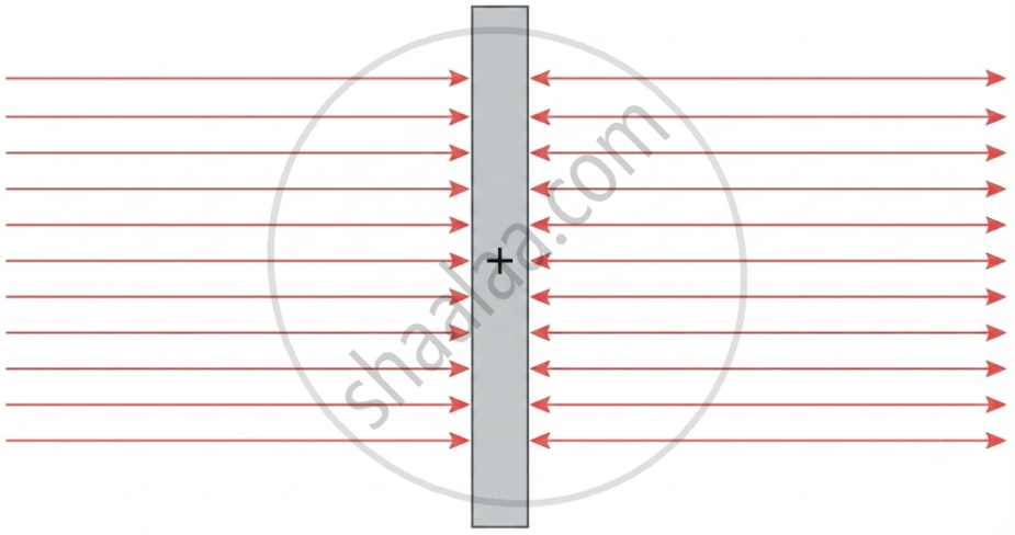
5. Charged Conducting Plate: This diagram shows a large, flat, charged conducting plate. Since the plate is a conductor, the charge distributes itself uniformly (on both surfaces, though only one is fully visible here). The resulting electric field lines are perpendicular to the surface of the plate and are uniformly spaced, indicating a constant electric field strength near the surface.
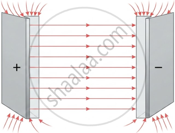
6. Parallel Plate Capacitor: This final diagram visualises the most uniform practical electric field: a parallel plate capacitor. It consists of two large, closely spaced conducting plates carrying equal and opposite charges. In the central region between the plates, the electric field lines are parallel and equally spaced, representing a nearly uniform field. Near the edges of the plates, the field lines curve outward, a phenomenon known as "fringing."
Example
Setup
The example uses three sets of electric field line diagrams to test how the number and density of field lines reveal charge sign, relative magnitude, and field strength at specific points.
(i) Sign and ratio of two charges
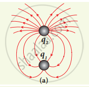 Since field lines start on positive charges and end on negative charges, q2 (source of 18 lines) is positive and q1 (receiving 6 lines) is negative. The ratio is found using the line cne count: \[\begin{vmatrix} \frac{q_1}{q_2} \end{vmatrix}=\frac{N_1}{N_2}=\frac{6}{18}=\frac{1}{3}\], meaning ∣q2∣ = 3∣q1∣ - q2 is three times stronger than q1.
(ii) Equal charges and field strength at three points
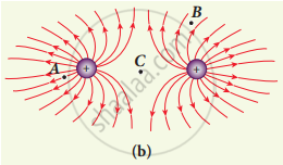 Both charges are positive and equal in magnitude, since each emits the same number of lines (N = 18). Point A sits where lines are denser, so the field there is stronger than at point B, where lines are more spread out. Point C has no lines passing through it at all, meaning the two fields exactly cancel there — the resultant field is zero.shaalaa
(iii) Three charges, solving for q1 and q3
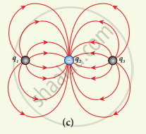 Lines start at q1 and q3 and end at q2, so q1 and q3 are positive while q2 is negative. Using the the line-count ratio: \[\begin{vmatrix} \frac{q_1}{q_2} \end{vmatrix}=\frac{8}{16}=\frac{1}{2}= \begin{vmatrix} \frac{q_3}{q_2} \end{vmatrix}\], so q1 and q3 are each half the magnitude of q2. Given q2 = –20 nC, this gives q1 = q3 = +10 nC.
Key takeaway
This example demonstrates the core principle that field-line count is proportional to charge magnitude, letting you compare or calculate unknown charges purely from a diagram, while line density at a point indicates local field strength (dense = strong, absent = zero).
Real-Life Analogy
Electric field lines behave like wind streamlines or water flow lines — you cannot see the wind or the field directly, but the lines show you the direction and relative strength of the flow at every point in space.