Topics
National Income and Related Aggregates
- Macroeconomics Vs Microeconomics
- Representative Goods and Sectors
- Macroeconomic Agents and Government Role
- Emergence of Macroeconomics
- Context of the Present Book of Macroeconomics
- Meaning of Economic Wealth and Final Goods
- Stocks, Flows, and Depreciation
- Capital Formation, Trade-off & Circular Flow of Income
- Circular Flow of Income and Methods of Calculating National Income
- Output Method/Product Method
- Expenditure Method
- Income Method
- Factor Cost, Basic Prices and Market Prices
- Some Macroeconomic Identities
- National Disposable Income
- Private Income
- National Income Aggregates
- Real GDP and Nominal GDP
- GDP and Welfare
Introductory Macroeconomics
Introduction
- A Simple Economy
- Central Problems of an Economy
- Concepts of Production Possibility Frontier
- Organisation of Economic Activities
- Positive and Normative Economics
- Macroeconomics Vs Microeconomics
Development Experience (1947-90) and Economic Reforms since 1991
- India's Economy Before Independence
- Low Level of Economic Development Under the Colonial Rule
- Agricultural Sector in India
- Industrial Sector
- Foreign Trade of India
- Demographic Condition
- Occupational Structure
- Infrastructure
- Post-Independence Economic Systems and Planning
- Five Year Plans (FYP)
- Agriculture
- Industry and Trade
- Trade Policy: Import Substitution
- The 1991 Economic Crisis and Reforms
- Background of the New Economic Policy
- Liberalisation
- Privatisation
- Globalisation
- World Trade Organisation (WTO)
- Impact of the Economic Reforms
Money and Banking
- Concept of Money
- Functions of Money
- Demand for Money and Supply of Money
- Money Creation by Banking System
- Limits to Credit Creation and Money Multiplier
- Policy Tools To Control Money Supply
- Demand and Supply for Money : A Detailed Discussion
- The Transaction Motive
- The Speculative Motive
- Various Measures of Supply of Money
- Narrow and Broad Money
- Demonetisation
Theory of Consumer Behaviour
- Consumer Behaviour: The Problem of Choice
- Basic Concepts of Microeconomics > Utility
- Cardinal Approach (Utility Analysis)
- Derivation of Demand Curve in the Case of a Single Commodity
- Ordinal Utility Analysis/Indifference Curve Analysis
Indian Economic Development
Current Challenges Facing Indian Economy
- Concept of Human Capital
- Sources of Human Capital
- Human Capital and Economic Growth
- Human Capital and Human Development
- State of Human Capital Formation in India
- Growth of Education Sector in India
- Challenges and Future Prospects in Education
- Rural Development in India
- Credit and Marketing in Rural Areas
- Agricultural Market System
- Diversification into Productive Activities
- Sustainable Development and Organic Farming
- The Nature and Importance of Work in Society
- Workers and Employment
- Participation of People in Employment
- Self-employed and Hired Workers
- Employment in Firms, Factories and Offices
- Growth and Changing Structure of Employment
- Informalisation of Indian Workforce
- Concept of Unemployment
- Government and Employment Generation
- Environment and Sustainable Development in India
- State of India’s Environment
- Concept of Sustainable Development
- Strategies for Sustainable Development
Development Experience of India – a Comparison with Neighbours
Determination of Income and Employment
- Aggregate Demand and Its Components
- Consumption
- Investment
- Determination of Income in Two-sector Model
- Determination of Equilibrium Income in the Short Run
- Macroeconomic Equilibrium with Price Level Fixed
- Effect of an Autonomous Change in Aggregate Demand on Income and Output
- The Multiplier Mechanism
- Paradox of Thrift
- Equilibrium Output and Employment
Introductory Microeconomics
Production and Costs
- Production Function
- Concept of Production
- Some Basic Concepts - Total, Average and Marginal Physical Products
- Relation Between Total, Average and Marginal Product
- Law of Variable Proportions
- Average and Marginal Physical Products
- Changes in Production
- Fixed Cost and Variable Cost
- Behaviour of Cost in the Short - Run
- Relationship Between Average Variable Cost and Average Total Cost and Marginal Cost
- Opportunity Cost
- Revenue Concepts
- Producer's Equilibrium
- Law of Supply
- Supply Schedule
- Distinction Between Supply and Stock
- Determinants of Supply
- Movement Along the Supply Curve Or Expansion and Contraction of Supply
- Measurement of Elasticity of Supply > Percentage Method
- Methods of Measurement of National Income
- Marginal Cost (MC)
- The Law of Diminishing Marginal Product
- Shapes of Product Curves
- Costs in Long Run Period
- Returns to Scale
Government Budget and the Economy
The Theory of the Firm Under Perfect Competition
- Concept of Market
- Market Equilibrium
- Determination of Market Equilibrium
- Effects of Changes (Shifts) in Demand on Equilibrium Price and Equilibrium Quantity
- Perfect Competition
- Imperfect Competition
- Factors Determining Market Forms
- Oligopoly
- Market Forms - Perfect Oligopoly
- Market Forms - Imperfect Oligopoly
- Equilibrium Price
- Applications of Tools of Demand and Supply Price Control
- Price Ceiling
- Price Floor
- Revenue Concepts
- Profit Maximisation Objective
- Determinants of a Firm’s Supply Curve
- Supply Schedule
- Price Elasticity of Supply
Balance of Payments
- Open Economy and Its Linkages
- Concept of Balance of Payments
- Current Account
- Capital Account
- Balance of Payments Surplus and Deficit
- Foreign Exchange Market
- Foreign Exchange Rate
- Determination of the Exchange Rate
- Merits and Demerits of Flexible and Fixed Exchange Rate Systems
- Managed Floating Exchange Rate System
Market Equilibrium
- Simple Monopoly in the Commodity Market
- Other Non - Perfectly Competitive Markets
Key Terms
- Disposable Income - Income remaining with households after paying taxes: \[Y_D = Y - T\]
- Marginal Propensity to Consume (c) - The fraction of additional income that a household spends on consumption.
- Automatic Stabiliser - A fiscal mechanism (like proportional taxes or transfers) that automatically reduces fluctuations in GDP without any new policy action.
Effect of a Tax Cut
- A cut in taxes ↑ disposable income (\[Y - T\])
- Higher disposable income ↑ consumption, which ↑ aggregate expenditure.
- The aggregate expenditure curve shifts upward by \[c \times \Delta T\].
- Result: National income (output) increases.
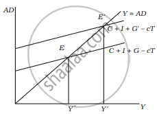
Effect of Higher Government Expenditure
Formula: Tax Multiplier
\[\frac{\Delta Y}{\Delta T} = \frac{-c}{1-c}\]
Formula: Government Expenditure Multiplier
\[\frac{\Delta Y}{\Delta G} = \frac{1}{1-c}\]
Formula: Balanced Budget Multiplier
\[\frac{\Delta Y}{\Delta G} = 1 \quad \text{when } \Delta G = \Delta T\]
Formula: Transfer Multiplier
\[\frac{\Delta Y}{\Delta TR} = \frac{c}{1-c}\]
Symbol Key
- \[\Delta Y\] = Change in national income
- \[\Delta T\] = Change in taxes
- \[\Delta G\] = Change in government expenditure
- \[\Delta TR\] = Change in transfer payments
- \[c\] = Marginal propensity to consume
Comparing the Multipliers
| Multiplier | Formula | Sign | Relative Size |
|---|---|---|---|
| Government Expenditure Multiplier | \(\frac{1}{1-c}\) | Positive | Largest |
| Transfer Multiplier | \(\frac{c}{1-c}\) | Positive | Smaller than Government Expenditure Multiplier |
| Tax Multiplier | \(\frac{-c}{1-c}\) | Negative | Smaller in absolute value than Government Expenditure Multiplier |
Balanced Budget Multiplier
- When the government increases both spending and taxes by the same amount (\(\Delta G = \Delta T\)), the net effect on income is still positive.
- The balanced budget multiplier = 1.
- Income rises by exactly the amount of the increase in government spending.
Proportional Taxes
- Fixed tax: (T) (lump sum)
- Proportional tax: (T = tY), where (t) = tax rate.
- Disposable income becomes: \[(1-t)Y\]
Effect on the economy:
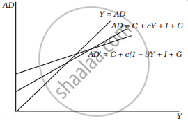
Government and Aggregate Demand (proportional taxes make the AD schedule flatter)
- Makes the AD (Aggregate Demand) schedule flatter.
- Reduces the value of the multiplier.
- Acts as an automatic stabiliser.
Automatic Stabilisers
- Proportional income taxes and transfers automatically reduce economic fluctuations.
- During a boom: GDP ↑ → tax collection ↑ → disposable income rises by less → consumption spending is dampened.
- During a recession: GDP ↓ → taxes ↓ → disposable income is cushioned → fall in consumption is reduced.
- No new policy needed — the system corrects itself.
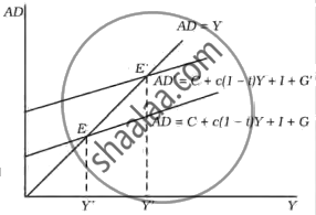
Increase in Government Expenditure (with proportional taxes)
Transfer Payments
- Government transfers raise household income, but only a fraction \(c\) is spent.
- Transfer multiplier \(\frac{c}{1-c}\) is smaller than the government expenditure multiplier \(\frac{1}{1-c}\).
- Reason: Direct govt. spending adds fully to demand; transfers add only the consumed portion.
Example 1
Given: Marginal Propensity to Consume (c = 0.8)
| Multiplier | Calculation | Value |
|---|---|---|
| Government Expenditure Multiplier | \(\frac{1}{1-0.8}\) | 5 |
| Tax Multiplier | \(\frac{-0.8}{1-0.8}\) | −4 |
Observation: The tax multiplier (–4) is smaller in magnitude than the govt. expenditure multiplier (5).
Example 2
Given: Marginal Propensity to Consume (c = 0.8), tax rate (t = 0.25)
\[c(1-t) = 0.8(1-0.25) = 0.8 \times 0.75 = 0.60\]
Government expenditure multiplier with proportional taxes:
\[\frac{1}{1-c(1-t)} = \frac{1}{1-0.60} = \frac{1}{0.40} = 2.5\]
If government expenditure rises by 100, output rises by:
\[2.5 \times 100 = 250\]
This is smaller than the increase in output with lump-sum taxes.
Example 3
Given: Marginal Propensity to Consume (c = 0.75)
When government purchases increase by 20:
\[\Delta Y = \frac{1}{1-0.75}\Delta G = 4 \times 20 = 80\]
When transfers increase by 20:
\[\Delta Y = \frac{0.75}{1-0.75}\Delta TR = 3 \times 20 = 60\]
Thus, income increases by less than it increased with a rise in government purchases.
Key Points: Changes in Taxes
- A tax cut raises disposable income and shifts aggregate expenditure up by \(c \times \Delta T\), increasing output.
- The tax multiplier is negative and smaller in absolute value than the govt. expenditure multiplier.
- The balanced budget multiplier = 1 - equal increases in G and T still raise income.
- Proportional taxes flatten the AD curve and lower the multiplier value.
- Proportional taxes and transfers act as automatic stabilisers - they cushion GDP swings without new policy action.
- The transfer multiplier is positive but smaller than the expenditure multiplier, as only a fraction of transfers is spent.
