Topics
Mathematical Logic
- Statements and Truth Values in Mathematical Logic
- Logical Connectives
- Tautology, Contradiction, and Contingency
- Quantifier, Quantified and Duality Statements in Logic
- Negations of Compound Statements
- Converse, Inverse, and Contrapositive
- Algebra of Statements
- Application of Logic to Switching Circuits
- Overview of Mathematical Logic
Matrices
- Elementry Transformations
- Adjoint and Inverse of a Matrix
- Application of Matrices
- Overview of Matrices
Trigonometric Functions
- Trigonometric Equations and Their Solutions
- Solutions of Triangle>Polar Co-Ordinates
- Solving a Triangle>Solving a Triangle
- Basics of Inverse Trigonometric Functions
- Graphs of Inverse Trigonometric Functions
- Domain, Range & Principal Value
- Properties of Inverse Trigonometric Functions > Self-adjusting Property
- Overview of Trigonometric Functions
- Properties of Inverse Trigonometric Functions > Reciprocal Property
- Properties of Inverse Trigonometric Functions > Complementary Property
- Properties of Inverse Trigonometric Functions > Addition & Subtraction Formula for Inverse Tangent
- Properties of Inverse Trigonometric Functions > Double-angle Property
- Properties of Inverse Trigonometric Functions > Triple-angle Property
- Properties of Inverse Trigonometric Functions > Addition–Subtraction Formula for Inverse Sine & Cosine
- Properties of Inverse Trigonometric Functions > Negative Argument Property
Pair of Straight Lines
Vectors
- Overview of Vectors
- Basic Concepts of Vector Algebra
- Types of Vectors in Algebra
- Algebra of Vectors > Scalar Multiplication
- Algebra of Vectors > Addition & Subtraction of Two Vectors
- Collinearity and Coplanarity of Vectors
- Vectors in Coordinate Geometry
- Components of Vector in Algebra
- Vector Joining Two Points in Algebra
- Section Formula in Vector Algebra
- Product of Two Vectors > Scalar (Dot) Product
- Product of Two Vectors > Vector (Cross) Product
- Direction Ratios, Direction Cosine & Direction Angles in Vector
- Scalar Triple Product
- Vector Triple Product
Line and Plane
Linear Programming
Differentiation
- Introduction & Derivatives of Some Standard Functions
- Derivatives of Composite Functions
- Geometrical Meaning of Derivative
- Derivative of Inverse Trigonometric Function
- Logarithmic Differentiation
- Differentiation of Implicit Functions
- Derivatives of Functions in Parametric Forms
- Higher Order Derivatives
- Overview of Differentiation
Applications of Derivatives
Indefinite Integration
Definite Integration
- Definite Integral as Limit of Sum
- Integral Calculus
- Methods of Evaluation and Properties of Definite Integral
- Overview of Definite Integration
Application of Definite Integration
- Application of Definite Integration
- Area Bounded by Two Curves
- Overview of Application of Definite Integration
Differential Equations
- Basic Concepts of Differential Equations
- Order and Degree of a Differential Equation
- Formation of Differential Equations
- Forms of Solving Differential Equations> Homogeneous Differential Equations
- Forms of Solving Differential Equations>Linear Differential Equations
- Applications of Differential Equation
- Solution of a Differential Equation
- Overview of Differential Equations
Probability Distributions
- Random Variables
- Probability Distribution of Discrete Random Variables
- Probability Distribution of a Continuous Random Variable
- Variance of a Random Variable
- Expected Value and Variance of a Random Variable
- Overview of Probability Distributions
Binomial Distribution
Introduction
Linear Programming Problem (LPP) is a method used to find the maximum or minimum value of a linear function under given linear constraints. In mathematics, the graphical method is used when the LPP involves two variables, because the constraints can be represented on a graph and the feasible region can be identified visually.
Important Definitions
| Term | Definition |
| Feasible Solution | A feasible solution is any solution that satisfies all the constraints of the LPP, including non-negativity restrictions. |
| Feasible Region | The common region that satisfies all the constraints on the graph is called the feasible region. Every point inside or on this region represents a feasible solution. |
| Infeasible Solution | Any point that does not satisfy all the given constraints is an infeasible solution. |
| Optimal Solution | A feasible solution that gives the maximum or minimum value of the objective function is called the optimal solution. |
| Corner Point | A corner point is a vertex of the feasible region formed by the intersection of boundary lines. In the graphical method, these points are checked first to find the optimum value. |
| Bounded Region |
A feasible region that is enclosed within finite boundaries and does not extend indefinitely in any direction. |
| Unbounded Region |
A feasible region that extends indefinitely in one or more directions and is not completely enclosed by boundaries. |
Corner Point Method
The Corner Point Method is based on the Extreme Point Theorem, which states that the optimum solution of an LPP, if it exists, occurs at a corner point of the feasible region.
Steps:

Note:
- For a bounded feasible region, maximum and minimum values occur at corner points.
- For an unbounded feasible region, an optimum value may or may not exist.
Example 1
Solve graphically:
Maximise Z = 4x + y
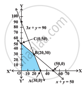
Subject to: \[x + y \leq 50\], \[3x + y \leq 90\], \[x \geq 0\], \[y \geq 0\].
Solution:
Step 1: Observe the type of region
The feasible region is the bounded region OABC. This is important because for a bounded feasible region, both maximum and minimum values exist at corner points.
Step 2: Identify the corner points
The corner points are (0, 0), (30, 0), (20, 30), and (0, 50). These are the only points that need to be checked for the maximum value.
Step 3: Evaluate Z at each corner point
| Corner Point | Value of Z = 4x + y |
|---|---|
| (0,0) | 0 |
| (30,0) | 120 |
| (20,30) | 110 |
| (0,50) | 50 |
Step 4: Conclude logically
The maximum value is 120 at (30, 0). This means that among all feasible solutions, the point (30, 0) gives the greatest value of the objective function.
Maharashtra State Board: Class 12
Key points: Methods to Solve LPP (Graphical / Corner Point Method)
-
An LPP is solved graphically when there are two variables.
-
The feasible region is formed by the common solution of all constraints.
-
The optimum value is found by evaluating the objective function at corner points.
-
If two corner points give the same optimum value, then all points on the joining segment are also optimal.
-
In an unbounded region, the required maximum or minimum may fail to exist.
-
If no feasible region exists, the LPP has no feasible solution.
Test Yourself
Shaalaa.com | Linear Programming part 2 (Graphical Method Thoerem 1)
Series: series 1
00:12:56 undefined
00:12:05 undefined
00:13:42 undefined
00:14:25 undefined
00:04:48 undefined
00:04:29 undefined
