Advertisements
Advertisements
Question
Solve the following problem :
The percentage of girls’ enrollment in total enrollment for years 1960-2005 is shown in the following table.
| Year | 1960 | 1965 | 1970 | 1975 | 1980 | 1985 | 1990 | 1995 | 2000 | 2005 |
| Percentage | 0 | 3 | 3 | 4 | 4 | 5 | 6 | 8 | 8 | 10 |
Fit a trend line to the above data by graphical method.
Advertisements
Solution
Taking year on X-axis and percentage of enrolment on Y-axis, we plot the points for enrolment corresponding to years. Joining these points, we get the graph of time series. We fit the trend line as shown in the following graph.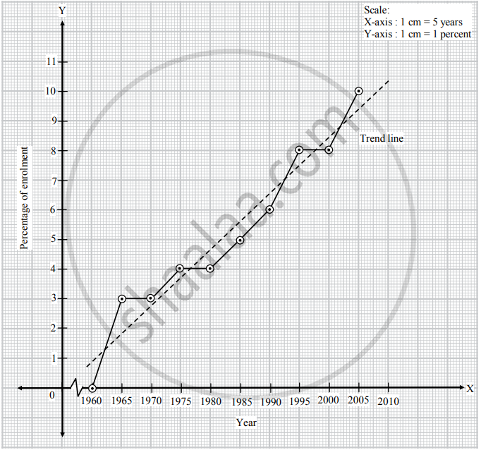
APPEARS IN
RELATED QUESTIONS
Obtain the trend line for the above data using 5 yearly moving averages.
Obtain the trend values for the data in using 4-yearly centered moving averages.
| Year | 1976 | 1977 | 1978 | 1979 | 1980 | 1981 | 1982 | 1983 | 1984 | 1985 |
| Index | 0 | 2 | 3 | 3 | 2 | 4 | 5 | 6 | 7 | 10 |
Fit a trend line to the data in Problem 7 by the method of least squares. Also, obtain the trend value for the year 1990.
Obtain the trend values for the above data using 3-yearly moving averages.
The simplest method of measuring trend of time series is ______.
Fill in the blank :
The method of measuring trend of time series using only averages is _______
State whether the following is True or False :
Graphical method of finding trend is very complicated and involves several calculations.
Solve the following problem :
The following table shows the production of pig-iron and ferro- alloys (‘000 metric tonnes)
| Year | 1974 | 1975 | 1976 | 1977 | 1978 | 1979 | 1980 | 1981 | 1982 |
| Production | 0 | 4 | 9 | 9 | 8 | 5 | 4 | 8 | 10 |
Fit a trend line to the above data by graphical method.
Fit a trend line to the following data by the method of least squares.
| Year | 1974 | 1975 | 1976 | 1977 | 1978 | 1979 | 1980 | 1981 | 1982 |
| Production | 0 | 4 | 9 | 9 | 8 | 5 | 4 | 8 | 10 |
Solve the following problem :
Following table shows the amount of sugar production (in lac tonnes) for the years 1971 to 1982.
| Year | 1971 | 1972 | 1973 | 1974 | 1975 | 1976 | 1977 | 1978 | 1979 | 1980 | 1981 | 1982 |
| Production | 1 | 0 | 1 | 2 | 3 | 2 | 3 | 6 | 5 | 1 | 4 | 10 |
Fit a trend line to the above data by graphical method.
Obtain trend values for the following data using 4-yearly centered moving averages.
| Year | 1971 | 1972 | 1973 | 1974 | 1975 | 1976 |
| Production | 1 | 0 | 1 | 2 | 3 | 2 |
| Year | 1977 | 1978 | 1979 | 1980 | 1981 | 1982 |
| Production | 3 | 6 | 5 | 1 | 4 | 10 |
Solve the following problem :
Fit a trend line to data by the method of least squares.
| Year | 1977 | 1978 | 1979 | 1980 | 1981 | 1982 | 1983 | 1984 |
| Number of boxes (in ten thousands) | 1 | 0 | 3 | 8 | 10 | 4 | 5 | 8 |
Solve the following problem :
Following table shows the number of traffic fatalities (in a state) resulting from drunken driving for years 1975 to 1983.
| Year | 1975 | 1976 | 1977 | 1978 | 1979 | 1980 | 1981 | 1982 | 1983 |
| No. of deaths | 0 | 6 | 3 | 8 | 2 | 9 | 4 | 5 | 10 |
Fit a trend line to the above data by graphical method.
Solve the following problem :
Following table shows the all India infant mortality rates (per ‘000) for years 1980 to 2010.
| Year | 1980 | 1985 | 1990 | 1995 | 2000 | 2005 | 2010 |
| IMR | 10 | 7 | 5 | 4 | 3 | 1 | 0 |
Fit a trend line to the above data by graphical method.
Solve the following problem :
Obtain trend values for data in Problem 16 using 3-yearly moving averages.
Solve the following problem :
Following tables shows the wheat yield (‘000 tonnes) in India for years 1959 to 1968.
| Year | 1959 | 1960 | 1961 | 1962 | 1963 | 1964 | 1965 | 1966 | 1967 | 1968 |
| Yield | 0 | 1 | 2 | 3 | 1 | 0 | 4 | 1 | 2 | 10 |
Fit a trend line to the above data by the method of least squares.
The complicated but efficient method of measuring trend of time series is ______
The simplest method of measuring trend of time series is ______
State whether the following statement is True or False:
Moving average method of finding trend is very complicated and involves several calculations
State whether the following statement is True or False:
Least squares method of finding trend is very simple and does not involve any calculations
The following table gives the production of steel (in millions of tons) for years 1976 to 1986.
| Year | 1976 | 1977 | 1978 | 1979 | 1980 | 1981 | 1982 | 1983 | 1984 | 1985 | 1986 |
| Production | 0 | 4 | 4 | 2 | 6 | 8 | 5 | 9 | 4 | 10 | 10 |
Obtain the trend value for the year 1990
Obtain the trend values for the data, using 3-yearly moving averages
| Year | 1976 | 1977 | 1978 | 1979 | 1980 | 1981 |
| Production | 0 | 4 | 4 | 2 | 6 | 8 |
| Year | 1982 | 1983 | 1984 | 1985 | 1986 | |
| Production | 5 | 9 | 4 | 10 | 10 |
Obtain trend values for data, using 3-yearly moving averages
Solution:
| Year | IMR | 3 yearly moving total |
3-yearly moving average (trend value) |
| 1980 | 10 | – | – |
| 1985 | 7 | `square` | 7.33 |
| 1990 | 5 | 16 | `square` |
| 1995 | 4 | 12 | 4 |
| 2000 | 3 | 8 | `square` |
| 2005 | 1 | `square` | 1.33 |
| 2010 | 0 | – | – |
Fit equation of trend line for the data given below.
| Year | Production (y) | x | x2 | xy |
| 2006 | 19 | – 9 | 81 | – 171 |
| 2007 | 20 | – 7 | 49 | – 140 |
| 2008 | 14 | – 5 | 25 | – 70 |
| 2009 | 16 | – 3 | 9 | – 48 |
| 2010 | 17 | – 1 | 1 | – 17 |
| 2011 | 16 | 1 | 1 | 16 |
| 2012 | 18 | 3 | 9 | 54 |
| 2013 | 17 | 5 | 25 | 85 |
| 2014 | 21 | 7 | 49 | 147 |
| 2015 | 19 | 9 | 81 | 171 |
| Total | 177 | 0 | 330 | 27 |
Let the equation of trend line be y = a + bx .....(i)
Here n = `square` (even), two middle years are `square` and 2011, and h = `square`
The normal equations are Σy = na + bΣx
As Σx = 0, a = `square`
Also, Σxy = aΣx + bΣx2
As Σx = 0, b = `square`
Substitute values of a and b in equation (i) the equation of trend line is `square`
To find trend value for the year 2016, put x = `square` in the above equation.
y = `square`
Complete the table using 4 yearly moving average method.
| Year | Production | 4 yearly moving total |
4 yearly centered total |
4 yearly centered moving average (trend values) |
| 2006 | 19 | – | – | |
| `square` | ||||
| 2007 | 20 | – | `square` | |
| 72 | ||||
| 2008 | 17 | 142 | 17.75 | |
| 70 | ||||
| 2009 | 16 | `square` | 17 | |
| `square` | ||||
| 2010 | 17 | 133 | `square` | |
| 67 | ||||
| 2011 | 16 | `square` | `square` | |
| `square` | ||||
| 2012 | 18 | 140 | 17.5 | |
| 72 | ||||
| 2013 | 17 | 147 | 18.375 | |
| 75 | ||||
| 2014 | 21 | – | – | |
| – | ||||
| 2015 | 19 | – | – |
Following table shows the amount of sugar production (in lakh tonnes) for the years 1931 to 1941:
| Year | Production | Year | Production |
| 1931 | 1 | 1937 | 8 |
| 1932 | 0 | 1938 | 6 |
| 1933 | 1 | 1939 | 5 |
| 1934 | 2 | 1940 | 1 |
| 1935 | 3 | 1941 | 4 |
| 1936 | 2 |
Complete the following activity to fit a trend line by method of least squares:
