Advertisements
Advertisements
Question
Solve the following problem :
Following table shows the number of traffic fatalities (in a state) resulting from drunken driving for years 1975 to 1983.
| Year | 1975 | 1976 | 1977 | 1978 | 1979 | 1980 | 1981 | 1982 | 1983 |
| No. of deaths | 0 | 6 | 3 | 8 | 2 | 9 | 4 | 5 | 10 |
Fit a trend line to the above data by graphical method.
Advertisements
Solution
Taking year on X-axis and number of deaths on Y-axis, we plot the points for number of deaths corresponding to year. Joining these points we get the graph of time series, we fit the trend line as shown in the following graph.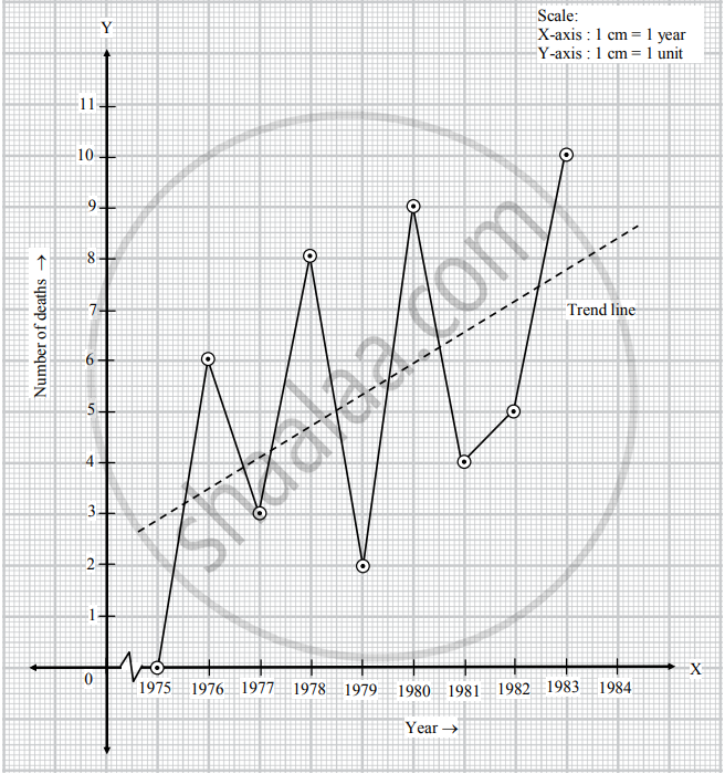
APPEARS IN
RELATED QUESTIONS
Obtain the trend line for the above data using 5 yearly moving averages.
Fit a trend line to the data in Problem 4 above by the method of least squares. Also, obtain the trend value for the index of industrial production for the year 1987.
Fit a trend line to the data in Problem 7 by the method of least squares. Also, obtain the trend value for the year 1990.
Obtain the trend values for the above data using 3-yearly moving averages.
Choose the correct alternative :
Which of the following is a major problem for forecasting, especially when using the method of least squares?
Choose the correct alternative :
What is a disadvantage of the graphical method of determining a trend line?
Fill in the blank :
The complicated but efficient method of measuring trend of time series is _______.
State whether the following is True or False :
Least squares method of finding trend is very simple and does not involve any calculations.
Fit a trend line to the following data by the method of least squares.
| Year | 1974 | 1975 | 1976 | 1977 | 1978 | 1979 | 1980 | 1981 | 1982 |
| Production | 0 | 4 | 9 | 9 | 8 | 5 | 4 | 8 | 10 |
Solve the following problem :
Obtain trend values for the following data using 5-yearly moving averages.
| Year | 1974 | 1975 | 1976 | 1977 | 1978 | 1979 | 1980 | 1981 | 1982 |
| Production | 0 | 4 | 9 | 9 | 8 | 5 | 4 | 8 | 10 |
Solve the following problem :
Fit a trend line to data in Problem 4 by the method of least squares.
Solve the following problem :
The percentage of girls’ enrollment in total enrollment for years 1960-2005 is shown in the following table.
| Year | 1960 | 1965 | 1970 | 1975 | 1980 | 1985 | 1990 | 1995 | 2000 | 2005 |
| Percentage | 0 | 3 | 3 | 4 | 4 | 5 | 6 | 8 | 8 | 10 |
Fit a trend line to the above data by graphical method.
Solve the following problem :
Obtain trend values for the data in Problem 7 using 4-yearly moving averages.
Following data shows the number of boxes of cereal sold in years 1977 to 1984.
| Year | 1977 | 1978 | 1979 | 1980 | 1981 | 1982 | 1983 | 1984 |
| No. of boxes in ten thousand | 1 | 0 | 3 | 8 | 10 | 4 | 5 | 8 |
Fit a trend line to the above data by graphical method.
Solve the following problem :
Obtain trend values for data in Problem 13 using 4-yearly moving averages.
Solve the following problem :
Obtain trend values for data in Problem 16 using 3-yearly moving averages.
The simplest method of measuring trend of time series is ______
The method of measuring trend of time series using only averages is ______
State whether the following statement is True or False:
Moving average method of finding trend is very complicated and involves several calculations
Following table shows the all India infant mortality rates (per ‘000) for years 1980 to 2010
| Year | 1980 | 1985 | 1990 | 1995 |
| IMR | 10 | 7 | 5 | 4 |
| Year | 2000 | 2005 | 2010 | |
| IMR | 3 | 1 | 0 |
Fit a trend line by the method of least squares
Solution: Let us fit equation of trend line for above data.
Let the equation of trend line be y = a + bx .....(i)
Here n = 7(odd), middle year is `square` and h = 5
| Year | IMR (y) | x | x2 | x.y |
| 1980 | 10 | – 3 | 9 | – 30 |
| 1985 | 7 | – 2 | 4 | – 14 |
| 1990 | 5 | – 1 | 1 | – 5 |
| 1995 | 4 | 0 | 0 | 0 |
| 2000 | 3 | 1 | 1 | 3 |
| 2005 | 1 | 2 | 4 | 2 |
| 2010 | 0 | 3 | 9 | 0 |
| Total | 30 | 0 | 28 | – 44 |
The normal equations are
Σy = na + bΣx
As, Σx = 0, a = `square`
Also, Σxy = aΣx + bΣx2
As, Σx = 0, b =`square`
∴ The equation of trend line is y = `square`
Fit equation of trend line for the data given below.
| Year | Production (y) | x | x2 | xy |
| 2006 | 19 | – 9 | 81 | – 171 |
| 2007 | 20 | – 7 | 49 | – 140 |
| 2008 | 14 | – 5 | 25 | – 70 |
| 2009 | 16 | – 3 | 9 | – 48 |
| 2010 | 17 | – 1 | 1 | – 17 |
| 2011 | 16 | 1 | 1 | 16 |
| 2012 | 18 | 3 | 9 | 54 |
| 2013 | 17 | 5 | 25 | 85 |
| 2014 | 21 | 7 | 49 | 147 |
| 2015 | 19 | 9 | 81 | 171 |
| Total | 177 | 0 | 330 | 27 |
Let the equation of trend line be y = a + bx .....(i)
Here n = `square` (even), two middle years are `square` and 2011, and h = `square`
The normal equations are Σy = na + bΣx
As Σx = 0, a = `square`
Also, Σxy = aΣx + bΣx2
As Σx = 0, b = `square`
Substitute values of a and b in equation (i) the equation of trend line is `square`
To find trend value for the year 2016, put x = `square` in the above equation.
y = `square`
Obtain the trend values for the following data using 5 yearly moving averages:
| Year | 2000 | 2001 | 2002 | 2003 | 2004 |
| Production xi |
10 | 15 | 20 | 25 | 30 |
| Year | 2005 | 2006 | 2007 | 2008 | 2009 |
| Production xi |
35 | 40 | 45 | 50 | 55 |
Following table shows the amount of sugar production (in lakh tonnes) for the years 1931 to 1941:
| Year | Production | Year | Production |
| 1931 | 1 | 1937 | 8 |
| 1932 | 0 | 1938 | 6 |
| 1933 | 1 | 1939 | 5 |
| 1934 | 2 | 1940 | 1 |
| 1935 | 3 | 1941 | 4 |
| 1936 | 2 |
Complete the following activity to fit a trend line by method of least squares:
The complicated but efficient method of measuring trend of time series is ______.
The publisher of a magazine wants to determine the rate of increase in the number of subscribers. The following table shows the subscription information for eight consecutive years:
| Years | 1976 | 1977 | 1978 | 1979 |
| No. of subscribers (in millions) |
12 | 11 | 19 | 17 |
| Years | 1980 | 1981 | 1982 | 1983 |
| No. of subscribers (in millions) |
19 | 18 | 20 | 23 |
Fit a trend line by graphical method.
Complete the following activity to fit a trend line to the following data by the method of least squares.
| Year | 1975 | 1976 | 1977 | 1978 | 1979 | 1980 | 1981 | 1982 | 1983 |
| Number of deaths | 0 | 6 | 3 | 8 | 2 | 9 | 4 | 5 | 10 |
Solution:
Here n = 9. We transform year t to u by taking u = t - 1979. We construct the following table for calculation :
| Year t | Number of deaths xt | u = t - 1979 | u2 | uxt |
| 1975 | 0 | - 4 | 16 | 0 |
| 1976 | 6 | - 3 | 9 | - 18 |
| 1977 | 3 | - 2 | 4 | - 6 |
| 1978 | 8 | - 1 | 1 | - 8 |
| 1979 | 2 | 0 | 0 | 0 |
| 1980 | 9 | 1 | 1 | 9 |
| 1981 | 4 | 2 | 4 | 8 |
| 1982 | 5 | 3 | 9 | 15 |
| 1983 | 10 | 4 | 16 | 40 |
| `sumx_t` =47 | `sumu`=0 | `sumu^2=60` | `square` |
The equation of trend line is xt= a' + b'u.
The normal equations are,
`sumx_t = na^' + b^' sumu` ...(1)
`sumux_t = a^'sumu + b^'sumu^2` ...(2)
Here, n = 9, `sumx_t = 47, sumu= 0, sumu^2 = 60`
By putting these values in normal equations, we get
47 = 9a' + b' (0) ...(3)
40 = a'(0) + b'(60) ...(4)
From equation (3), we get a' = `square`
From equation (4), we get b' = `square`
∴ the equation of trend line is xt = `square`
Following table gives the number of road accidents (in thousands) due to overspeeding in Maharashtra for 9 years. Complete the following activity to find the trend by the method of least squares.
| Year | 2008 | 2009 | 2010 | 2011 | 2012 | 2013 | 2014 | 2015 | 2016 |
| Number of accidents | 39 | 18 | 21 | 28 | 27 | 27 | 23 | 25 | 22 |
Solution:
We take origin to 18, we get, the number of accidents as follows:
| Year | Number of accidents xt | t | u = t - 5 | u2 | u.xt |
| 2008 | 21 | 1 | -4 | 16 | -84 |
| 2009 | 0 | 2 | -3 | 9 | 0 |
| 2010 | 3 | 3 | -2 | 4 | -6 |
| 2011 | 10 | 4 | -1 | 1 | -10 |
| 2012 | 9 | 5 | 0 | 0 | 0 |
| 2013 | 9 | 6 | 1 | 1 | 9 |
| 2014 | 5 | 7 | 2 | 4 | 10 |
| 2015 | 7 | 8 | 3 | 9 | 21 |
| 2016 | 4 | 9 | 4 | 16 | 16 |
| `sumx_t=68` | - | `sumu=0` | `sumu^2=60` | `square` |
The equation of trend is xt =a'+ b'u.
The normal equations are,
`sumx_t=na^'+b^'sumu ...(1)`
`sumux_t=a^'sumu+b^'sumu^2 ...(2)`
Here, n = 9, `sumx_t=68,sumu=0,sumu^2=60,sumux_t=-44`
Putting these values in normal equations, we get
68 = 9a' + b'(0) ...(3)
∴ a' = `square`
-44 = a'(0) + b'(60) ...(4)
∴ b' = `square`
The equation of trend line is given by
xt = `square`
