Topics
Commercial Mathematics
Compound Interest
- Compound Interest as a Repeated Simple Interest Computation with a Growing Principal
- Use of Compound Interest in Computing Amount Over a Period of 2 Or 3-years
- Use of Formula
- Finding CI from the Relation CI = A – P
Goods and Services Tax (G.S.T.)
Algebra
Banking
Geometry
Shares and Dividends
Linear Inequations
Mensuration
Quadratic Equations
Trigonometry
Ratio and Proportion
Statistics
Probability
Factorisation of Polynomials
- Function and Polynomial
- Division Algorithm for Polynomials
- Remainder Theorem
- Factor Theorem
- Applications of Factor Theorem
Matrices
Arithmetic and Geometric Progression
Co-ordinate Geometry
- Foundation of Coordinate Geometry
- Advanced Concept of Reflection in Mathematics
- Invariant Points
- Combination of Reflections
- Using Graph Paper for Reflection
Similarity
Symmetry
Loci
- Locus
- Points Equidistant from Two Given Points
- Points Equidistant from Two Intersecting Lines
- Summary of Important Results on Locus
- Important Points on Concurrency in a Triangle
Circles
Tangent and Secant Properties
Constructions
Area and Volume of Solids (Cylinder, Cone and Sphere)
- Mensuration of Cylinder
- Hollow Cylinder
- Mensuration of Cones
- Mensuration of a Sphere
- Hemisphere
- Conversion of Solids
- Solid Figures
- Problems on Mensuration
Trigonometrical Identities
Heights and Distances
- Angles of Elevation and Depression
- Problems based on Elevation and Depression
Statistics : basic concepts, Mean, Median, Mode. Histograms and Ogive
Probability
- Introduction
- Frequency Distribution & Data Arrangement
- Structure of a Frequency Distribution Table
- Example
- Real-life Applications
- Key Points Summary
Introduction
Data representation is the process of organizing and displaying raw data in a meaningful way so we can easily see patterns and draw conclusions.
The importance of representing data properly lies in helping us:
-
Understand large amounts of information quickly
-
Identify patterns and trends
-
Compare values easily
-
Make informed decisions based on facts
Frequency Distribution & Data Arrangement
Frequency Distribution:
It shows how many times each value appears in a dataset, making it much easier to work with large sets of numbers.
Arranging Data in Order:
Before we can create a frequency distribution, we need to arrange raw data in either:
1. Ascending Order – From smallest to largest value
-
Example: 10, 20, 30, 40, 50, 60, 70, 80
2. Descending Order – From largest to smallest value
-
Example: 80, 70, 60, 50, 40, 30, 20, 10
When data is arranged in ascending or descending order, it's called an array.
Structure of a Frequency Distribution Table
| Column 1 | Column 2 | Column 3 |
|---|---|---|
| Marks | Tally Marks | Number of Students (Frequency) |
-
Column 1 (Marks): All unique values from lowest to highest
-
Column 2 (Tally Marks): Visual representation using short lines (||||) to count
-
Column 3 (Frequency): The number count for each mark
Example
Problem: Construct a frequency distribution table for the following data:
Raw data: 55, 56, 56, 54, 57, 57, 56, 55, 55, 56, 56, 57, 55, 56, 56, 54, 56, 55, 54, 57, 57, 56, 55, 54, and 55.
Solution:
Step 1: Arrange data in ascending order
-
54, 54, 54, 54, 55, 55, 55, 55, 55, 55, 55, 56, 56, 56, 56, 56, 56, 56, 56, 56, 57, 57, 57, 57, 57
Step 2: Create the frequency distribution table
Step 3: Mark Tally for Each Value
Step 4: Count the Tally Marks
| Marks | Tally Marks | Frequency |
|---|---|---|
| 54 | |||| | 4 |
| 55 | `cancel (||||)` || | 7 |
| 56 | `cancel (||||)` ||| | 9 |
| 57 | `cancel (||||)` | 5 |
| Total | 25 |
Real-life Applications
Here are some practical uses of frequency distribution in everyday life.
1. School Test Results
-
Teachers use frequency distribution to analyse test scores and see how many students fall into different performance ranges (excellent, good, average, etc.)
2. Election Polling
-
Election officials count votes using tally marks and create frequency distributions to see how many people voted for each candidate
3. Quality Control in Manufacturing
-
Factories use frequency distribution to check products—how many items are defective, how many are perfect, how many need minor adjustments
4. Medical Records
-
Hospitals organise patient data like blood pressure readings, ages, or weights using frequency distribution to identify common health patterns


Key Points Summary
-
Array is raw data arranged in ascending or descending order of magnitude.
-
Frequency distribution shows how many times each value appears in a dataset.
-
A frequency distribution table has three columns: marks, tally marks, and frequency.
-
Tally marks are visual counting tools; every fifth mark is drawn as a diagonal cross (`cancel (||||)`).
-
Arranging data in order makes it easier to count frequencies accurately.
Test Yourself
Video Tutorials
Shaalaa.com | Graphical Representation of Data
Related QuestionsVIEW ALL [95]
Draw frequency polygons for each of the following frequency distribution:
(a) using histogram
(b) without using histogram
|
C.I |
10 - 30 |
30 - 50 |
50 - 70 | 70 - 90 | 90 - 110 | 110 - 130 | 130 - 150 |
| ƒ | 4 | 7 | 5 | 9 | 5 | 6 | 4 |
The marks obtained (out of 100) by a class of 80 students are given below:
| Marks | Number of students |
| 10 – 20 | 6 |
| 20 – 30 | 17 |
| 30 – 50 | 15 |
| 50 – 70 | 16 |
| 70 – 100 | 26 |
Construct a histogram to represent the data above.
Students of a small school use different modes of travel to school as shown below:
| Mode | Bus | Car | Bicycle | Auto | On foot |
| No. of students | 142 | 98 | 50 | 34 | 16 |
Draw a suitable bar graph.
Construct a frequency polygon for the following distribution:
| Class-intervals | 0-4 | 4 - 8 | 8 - 12 | 12 - 16 | 16 - 20 | 20 - 24 |
| Frequency | 4 | 7 | 10 | 15 | 11 | 6 |
Following table shows a frequency distribution for the speed of cars passing through at a particular spot on a high way:
| Class interval (km/h) | Frequency |
| 30 – 40 | 3 |
| 40 – 50 | 6 |
| 50 – 60 | 25 |
| 60 – 70 | 65 |
| 70 – 80 | 50 |
| 80 – 90 | 28 |
| 90 – 100 | 14 |
Draw the frequency polygon representing the above data without drawing the histogram.
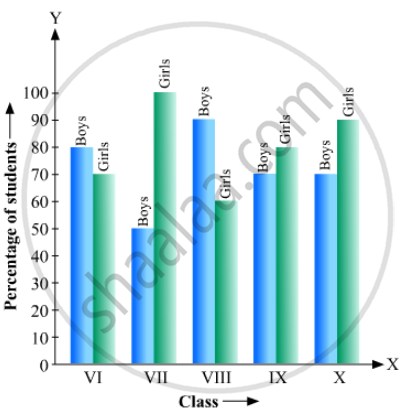
Given below are the seats won by different political parties in the polling outcome of a state assembly elections:-
| Political Party | A | B | C | D | E | F |
| Seats Won | 75 | 55 | 37 | 29 | 10 | 37 |
- Draw a bar graph to represent the polling results.
- Which political party won the maximum number of seats?
