Definitions [10]
Define production function.
A production function indicates the highest amount of a product that can be made in a specific time frame using a set amount of inputs, utilising the best available production method.
A production function shows the maximum quantity of a commodity that can be produced per unit of time with the given amount of inputs when the best production technique available is used. A production function can be expressed in the form of a table, graph or algebraic equation. In the form of an algebraic equation, the production function for a good may be expressed as:
QX = f(F1, F2...Fn) Where OX is the quantity of output of the commodity X: and F1, F2 ... Fn are the quantities of different inputs used to produce the commodity X.
Older definitions: Production is making material goods.
Newer (economic) definitions: Production is creating value for sale or paid services.
- Fraser: “Production means—putting utility into.”
- Cairncross: “Making goods for sale or rendering paid services.”
- Meyers: “Any activity resulting in goods/services meant for exchange.”
- “As the proportion of the factor in a combination of factors is increased after a point, first the marginal and then the average product of that factor will diminish.”
—Benham - “The law of variable proportion states that if the inputs of one resource is increased by equal increment per unit of time while the inputs of other resources are held constant, total output will increase, but beyond some point the resulting output increases will become smaller and smaller.”
—Leftwich - “An increase in some inputs relative to other fixed inputs will, in a given state of technology, cause output to increase; but after a point the extra output resulting from the same additions of extra inputs will become less and less.”
—Samuelson
- "The term returns to scale refers to the changes in output as all factors change by the same proportion." — Koutsoyiannis
- "Returns to scale relates to the behaviour of total output as all inputs are varied and is a long run concept." — Leibhafsky
Define variable cost.
Variable Cost refers to those costs which are incurred by a firm on the variable inputs for production. The variable costs are a positive function of output, i.e., as output increases, variable costs also increase and vice versa.
"The law of supply states that the higher the price, the greater the quantity supplied or the lower the price, the smaller the quantity supplied." – Dooley
"The long run average cost curve shows the lowest average cost of producing output when all inputs can be varied freely." - Robert Awh
"Long-run marginal cost curve is that which shows the extra cost incurred in producing one more unit of output when all inputs can be changed." - Robert Awh
"The long run total cost of production is the least possible cost of producing any given level of output when all inputs are variable." - Libhafasky
- "In the long-run, all the factors of production are assumed to be variable." - Koutsoyiannis
- "It will be helpful to think of the long run situation into any one in which the firm can move." - Leftwich
Formulae [3]
A production function can be shown as:
- A table (showing different combinations of inputs and output),
- A graph, or
- An equation (algebraic form).
General form:
\[Q_x=f(f_1,f_2,\ldots,f_n)\]
Where:
- Qx = quantity of output of commodity X,
- f1, f2,…, fn = quantities of different factor inputs,
- Qx is the dependent variable (depends on inputs) ,
- f1, f2,…, fn are independent variables.
If we assume only two inputs: labour (L) and capital (K):
\[Q_x=f(L,K)\]
Where:
-
P: Price of the commodity
-
I: Input prices
-
T: Technology
-
N: Number of sellers
-
G: Government policy
-
E: Expectations
-
R: Related goods prices
-
F: Natural factors
-
Tr: Transport/communication
\[MC_n=TC_n-TC_{n-1}\]
Where:
- MCn: Marginal cost of nth unit
- TCn: Total cost at n units
- TCn−1: Total cost at (n-1) units
Or, more generally:
\[MC=\frac{\Delta TC}{\Delta Q}\]
- ΔTC: Change in total cost
- ΔQ: Change in quantity of output (usually 1 unit)
Theorems and Laws [5]
Explain the law of variable proportions with the help of a diagram.
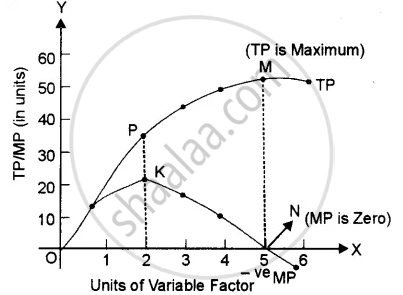
The law of variable proportions (LVP) states that as we increase the quantity of only one input, keeping other inputs fixed, total product (TP) initially increases at an increasing rate, then at a decreasing rate and finally at a negative rate.
In the given diagram, the quantity of the variable factor has been measured on X-axis and the Y-axis measures the total product on the Y-axis. The diagram indicates how the total product and marginal product change as a result of increases in the quantity of one factor to a fixed quantity of other factors.
The law can be better explained through three stages:
- First stage:
- Increasing return to a factor: In the first stage, every additional variable factor adds more and more to the total output. It means TP increases at an increasing rate and the MP of each variable factor rises. Better utilisation of fixed factors and increases in the efficiency of a variable factor due to specialisation are the major factors responsible for increasing returns. The increasing returns to a factor stage have been shown in the given diagram between O to P. It implies. TP increases at an increasing rate (till point ‘P’) and MP rises till it reaches its maximum point ‘K,’ which marks the end of the first phase.
- Increasing return to a factor: In the first stage, every additional variable factor adds more and more to the total output. It means TP increases at an increasing rate and the MP of each variable factor rises. Better utilisation of fixed factors and increases in the efficiency of a variable factor due to specialisation are the major factors responsible for increasing returns. The increasing returns to a factor stage have been shown in the given diagram between O to P. It implies. TP increases at an increasing rate (till point ‘P’) and MP rises till it reaches its maximum point ‘K,’ which marks the end of the first phase.
- Second stage:
- Diminishing returns to a Factor: In the second stage, every additional variable factor adds a lesser and lesser amount of output. It means TP increases at a diminishing rate and MP falls with an increase in a variable factor. The breaking of the optimum combination of a fixed and variable factor is the major factor responsible for diminishing returns. The second stage ends at point ‘S’ when MP is zero and TP is maximum (point ‘M’).
Stage 2 is very crucial, as a rational producer will always aim to produce in this phase because TP is maximum and MP of each variable factor is positive.
- Diminishing returns to a Factor: In the second stage, every additional variable factor adds a lesser and lesser amount of output. It means TP increases at a diminishing rate and MP falls with an increase in a variable factor. The breaking of the optimum combination of a fixed and variable factor is the major factor responsible for diminishing returns. The second stage ends at point ‘S’ when MP is zero and TP is maximum (point ‘M’).
- Third stage:
- Negative Returns to a Factor: In the third stage the employment of additional variable factors causes TP to decline. MP now becomes negative. Therefore, this stage is known as negative returns to a factor. Poor coordination between variable and fixed factors is the basic cause for this stage. In the fig., the third stage starts after point ‘N’ on the MP curve and point ‘O’ on the TP curve. The MP of each variable factor is negative in the 3 stages. So, no firm would deliberately choose to operate in this stage.
- If you keep increasing the variable input (e.g., labour) for a fixed input (e.g., land), the total production goes up at first, then grows slowly, and finally can go down.
- Marginal product (extra output from one more unit) and average product (output per unit) also rise at first, but later start to fall.
State the law of supply.
The law of supply states that other factors being equal, the quantity of a good supplied increases with an increase in the price level and decreases with a decrease in the price level of a good.
Law of supply states the direct relationship between price and quantity supplied, keeping other factors constant.
The law of supply states that other factors being equal, the quantity of a good supplied increases with an increase in the price level and decreases with a decrease in the price level of a good.
The supply schedule below shows the positive relationship between price and quantity supplied.
| Price (in Rs) | Quantity Supplied |
| 5 | 100 |
| 10 | 200 |
| 15 | 300 |

SS is the supply curve sloping upwards. When the price increases from Rs. 5 to Rs. 15, the quantity supplied also increases from 100 units to 300 units.
Explain the law of supply.
The law of supply shows a direct relationship between the price of a good and the quantity supplied. As the price rises, the quantity supplied also increases. This scenario is represented by an upward-sloping supply curve. This happens mainly due to two reasons:
- Profit Motivation: When the price of a product goes up, the chance of earning more profit also increases (assuming other factors remain the same). This encourages producers to supply more of that product.
- Rising Production Costs: As production increases, the cost of making each additional unit (marginal cost) also rises. So, producers are willing to produce and supply more only if the price is high enough to cover these extra costs.
“Other things being constant, the higher the price of a commodity, more is the quantity supplied; and lower the price of a commodity, less is the quantity supplied.”
In simple words: When the price rises, supply rises; when the price falls, supply falls.
There is a direct relationship between price and quantity supplied.
Symbolically:
Sx = f (Px)
Where:
- S = Supply
- x = Commodity
- f = Function
- P = Price of the commodity
Key Points
- A production function shows the technical relationship between physical inputs and maximum possible output in a given time.
- Short run: At least one factor is fixed; the firm changes output by changing only variable factors.
- Long run: All factors are variable; the firm can change the scale of production and plant size.
- Short‑run production function Q = f (L) → study of returns to a factor and Law of Variable Proportions.
- Long‑run production function → study of returns to scale.
- Production is any process that adds value/utility for sale or exchange.
- All four factors (land, labour, capital, and organisation) must be balanced.
- Efficiency is when each factor’s extra contribution matches its cost.
- Services and goods are both considered production.
- TP increases first, gets maximum, then may fall.
- AP is average for each worker; it first rises, then falls.
- MP is the extra that comes from each new worker; it rises, then falls, and can become negative.
- Only one input is changed; others are fixed.
- First, output improves quickly.
- Later, output slows down and may decrease.
- Businesses use this law to find the best input mix.
- Short-run cost function splits costs into fixed & variable.
- Fixed costs do not change with output. Variable costs do.
- Graphs and tables make these concepts easier to remember.
- Extra revenue from selling one more unit
- MR = Change in Total Revenue
- Formula: MR = TRₙ − TRₙ₋₁
- Example: ₹4200 − ₹4000 = ₹200
- Producer’s equilibrium is the output level where the producer earns maximum profit and has no incentive to change output.
- Under the TR–TC approach, equilibrium occurs at the output where the vertical gap between TR and TC is greatest.
- Under the MR–MC approach, equilibrium occurs where MR = MC and MC is rising; MR > MC implies “increase output”, while MR < MC implies “decrease output”.
- Law of supply: The Higher the price, higher the supply; lower price, lower supply (if all else stays the same).
- Exceptions: rare items, short periods, perishable goods, some labor markets.
- Supply is always shown using a schedule (table) and a curve (graph).
- Supply schedule shows price and quantity supplied in tabular form
- Assumes other factors constant
- Types: Individual and Market
- Individual supply schedule shows supply of one producer
- Market supply schedule shows total supply of all producers
- Market supply = sum of individual supplies
- Law of supply: Higher price → higher quantity supplied
- Supply curve is graphical form of supply schedule
- Price on Y-axis, quantity on X-axis
- Supply curve slopes upward
- Types: Individual supply curve and Market supply curve
- Shows total quantity supplied by all producers at different prices.
- Market supply = sum of individual supplies (A + B + C).
- Higher price → higher market supply.
- Market supply curve slopes upward, showing direct relationship.
- National Income = Money value of final goods and services produced in one year.
- Circular Flow: Production → Income → Expenditure → Production.
- Output Method: Measures the value of final goods and services produced.
- Income Method: Adds wages, rent, interest, and profit.
- Expenditure Method: Adds spending on final goods and services; all three methods give the same national income.
- Marginal cost = extra cost for one extra unit.
- MC uses only variable costs (not fixed cost).
- MC curve is U-shaped in the short run.
- MC is key for decision making: output is optimal when Marginal Cost = Marginal Revenue.
- Sum of all MCs = Total Variable Cost (TVC).
- In the long run, firms can change all production factors for least cost.
- LAC curve helps in selecting the best way to produce for each output.
- LMC tells us how much extra cost is needed to raise output by one unit.
- Understanding cost curves helps firms plan profitably for both present and future production.
Important Questions [54]
- Define production function.
- Distinguish between short-run and long-run production functions.
- In What Circumstances May the Production Possibility Frontier Shift Away from the Origin? Explain.
- Explain the Central Problem of "Choice of Technique".
- Giving Reason Comment on the Shape of Production Possibilities Curve Based on the Following Schedule :
- What Will Be the Impact of Recently Launched 'Clean India Mission' (Swachh Bharat Mission) on the Production Possibilities Curve of the Economy and Why?
- What Will Likely Be the Impact of Large-scale Outflow of Foreign Capital on Production Possibilities Curve of the Economy and Why?
- Giving Reason Comment on the Production Possibilities Curve Based on the Following Schedule:
- Giving Reason Comment on the Shape of Production Possibilities Curve Based on the Following Schedule :
- What is Likely to Be the Impact of "Make in India" Appeal to the Foreign Investors by the Prime Minister of India, on the Production Possibilities Frontier of India? Explain
- Giving Reason Comment on the Shape of Production Possibilities Curve Based on the Following Schedule:
- What Will Be the Impact of "Education for All Campaign" (Sarv Shiksha Abhiyan) on The Production Possibilities Curve of the Indian Economy and Why?
- What Will Likely Be the Impact of the Large-scale Inflow of Foreign Capital in India on Production Possibilities Curve and Why?
- Why is Production Possibilities Curve Concave? Explain
- Why is a production possibilities curve downward sloping? Explain
- Explain the Central Problem of "What is Produced and in What Quantities.".
- Complete the Following Table
- State the relation between marginal product and average product. Show this relation in a diagram.
- Complete the Following Table:
- State Different Phases of the Law of Variable Proportions on the Basis of Total Product. Use Diagram
- State the Behaviour of Marginal Product in the Law of Variable Proportions. Explain the Causes of this Behaviour
- What Are the Different Phases in the Law of Variable Proportions in Terms of Total Product ? Give Reasons Behind Each Phase. Use Diagram.
- When the Average Product (Ap) is Maximum, the Marginal Product (Mp) Is: (Choose the Correct Alternative)
- From the Following Data Find Out the Level of Output that Will Give the Producer Maximum Profit (Use Marginal Cost and Marginal Revenue Approach,) Give Reasons For Your Answer
- What is the Behaviour of (A) Average Fixed Cost and (B) Average Variable Cost as More and More Units of a Good Are Produced?
- Define Cost. Distinguish Between Fixed and Variable Costs. Give One Example of Each.
- Give two examples of fixed costs.
- Define Fixed Cost. Give an Example.
- Define Variable Cost.
- Give two examples of variable costs.
- Define variable cost.
- Answer the Following Question. Explain the Relation Between the Average Variable Cost (Avc) Curve and the Marginal Cost (Mc) Curve. Use Diagram
- What Happens to the Difference Between Average Total Cost and Average Variable Cost as Production is Increased?
- State the Relation Between Mc Curve and Avc and Atc Curves.
- Which of the Following Statements Are True Or False? Give Valid Reasons in Support of Your Answer. Total Cost Curve and Total Variable Cost Curve Are Parallel to Each Other
- What is the Relation Between Marginal Cost and Average Variable Cost When Marginal Cost is Rising and Average Variable Cost is Falling?
- Draw Average Variable Cost, Average Total Cost ad Marginal Cost curves in a single diagram.
- What is the Relation Between Average Variable Cost and Average Total Cost, If Total Fixed Cost is Zero?
- What is Opportunity Cost? Explain with the Help of a Numerical Example.
- Explain the Concepts of Opportunity Cost and Marginal Rate of Transformation Using a Production Possibility Schedule Based on the Assumption that No Resource is Equally Efficient in Production of All Goods.
- Define Opportunity Cost.
- A Producer Starts a Business by Investing His Own Savings and Hiring the Labour. Identify Implicit and Explicit Costs from this Information. Explain.
- Which of the Following Does Not Cause Shift of Supply Curve of a Good?
- Explain the difference between "Shift of Supply Curve" and "Movement along Supply Curve". State one factor responsible for each. Use diagrams.
- Fill in the Blank. If the Market Supply of a Commodity X Changes Due to Improvement in Technology, the Market Supply Curve Will ___________.
- Fill in the Blank. If the Market Supply of a Commodity X Changes Due to a Rise in the Price of Factor Input, the Market Supply Curve Will ____________.
- What is 'Change in Supply'? Explain the Effect of Tax Imposed on a Good on the Supply Of The Good.
- When Does 'Shift' in Supply Curve Take Place?
- Choose the Correct Answer from Given Options If the Supply Curve is a Straight Line Parallel to the Vertical Axis (Y-axis), Supply of the Good is Called as _________.
- Total Revenue is Rs 400 When the Price of the Commodity is Rs 2 per Unit. When Price Rises to Rs 3 per Unit, the Quantity Supplied is 300 Units. Calculate the Price Elasticity of Supply
- Explain the Geometric Method of Measuring Price Elasticity of Supply. Use Diagram.
- The Price Elasticity of Supply of a Good is 0.8. Its Price Rises by 50 Percent. Calculate the Percentage Increase in Its Supply.
- Choose the Correct Alternative from Given Options: the Average Product Curve in the Input-output Plane, Will Be ____________.
- Which of the Following Statements Are True Or False? Give Valid Reasons in Support of Your Answer. Average Product Curve and Marginal Product Curves Are 'U-shaped' Curves.
Concepts [26]
- Production Function
- Basics of Production Theory
- Variation of Output in the Short-Run Returns to a Factor
- Relation Between Total, Average and Marginal Product
- Law of Variable Proportions
- Average and Marginal Physical Products
- Changes in Production
- Cost - Fixed Cost
- Cost -variable Cost
- Behaviour of Cost in the Short - Run
- Relationship Between Average Variable Cost and Average Total Cost and Marginal Cost
- Concept of Opportunity Cost
- Marginal Revenue
- Producer's Equilibrium
- Law of Supply
- Market Supply Schedule
- Distinguish between Stock and Supply
- Determinants of Supply
- Movements Along and Shifts in Supply Curve
- Measurement of Elasticity of Supply
- Methods of Measurement of National Income
- Cost Concepts > Marginal Cost
- The Law of Diminishing Marginal Product
- Shapes of Product Curves
- Costs in Long Run Period
- Returns to Scale
