Topics
Relations and Functions
Relations and Functions
Algebra
Inverse Trigonometric Functions
Matrices
- Concept of Matrices
- Types of Matrices
- Equality of Matrices
- Operations on Matrices> Addition and Subtraction of Matrices
- Operations on Matrices>Scalar Multiplication
- Operations on Matrices> Matrix Multiplication
- Transpose of a Matrix
- Symmetric and Skew Symmetric Matrices
- Invertible Matrices
- Overview of Matrices
Calculus
Determinants
Vectors and Three-dimensional Geometry
Continuity and Differentiability
- Continuous and Discontinuous Functions
- Algebra of Continuous Functions
- Concept of Differentiability
- Derivatives of Composite Functions
- Derivative of Implicit Functions
- Derivative of Inverse Function
- Exponential and Logarithmic Functions
- Logarithmic Differentiation
- Derivatives of Functions in Parametric Forms
- Second Order Derivative
- Overview of Continuity and Differentiability
Linear Programming
Probability
Applications of Derivatives
Integrals
- Introduction of Integrals
- Integration as an Inverse Process of Differentiation
- Properties of Indefinite Integral
- Methods of Integration> Integration by Substitution
- Methods of Integration>Integration Using Trigonometric Identities
- Methods of Integration> Integration Using Partial Fraction
- Methods of Integration> Integration by Parts
- Integrals of Some Particular Functions
- Definite Integrals
- Fundamental Theorem of Integral Calculus
- Evaluation of Definite Integrals by Substitution
- Properties of Definite Integrals
- Overview of Integrals
Sets
Applications of the Integrals
Differential Equations
- Basic Concepts of Differential Equations
- Order and Degree of a Differential Equation
- General and Particular Solutions of a Differential Equation
- Methods of Solving Differential Equations> Variable Separable Differential Equations
- Methods of Solving Differential Equations> Homogeneous Differential Equations
- Methods of Solving Differential Equations>Linear Differential Equations
- Overview of Differential Equations
Vectors
- Basic Concepts of Vector Algebra
- Direction Ratios, Direction Cosine & Direction Angles
- Types of Vectors in Algebra
- Algebra of Vector Addition
- Multiplication in Vector Algebra
- Components of Vector in Algebra
- Vector Joining Two Points in Algebra
- Section Formula in Vector Algebra
- Product of Two Vectors
- Overview of Vectors
Three - Dimensional Geometry
Linear Programming
Probability
Introduction
The Fundamental Theorem of Integral Calculus connects differentiation and integration. It shows that a definite integral can be evaluated by finding an antiderivative of the given function and using the values at the upper and lower limits.
It turns area-based integral ideas into a quick calculation method used in board and entrance examinations.
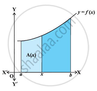
Definition: Area Function
If a function f is continuous on an interval, the area function is defined by
This means that A(x) gives the area accumulated from x = a to a variable point x.
Maharashtra State Board: Class 12
Theorem: First Fundamental Theorem
If f is continuous on [a, b] and
Theorem: Second Fundamental Theorem
If f is continuous on [a, b] and F is any antiderivative of f, then
This is the formula most often used in exams to evaluate definite integrals.
Example 1
\[\int_{4}^{9} \frac{\sqrt{x}}{(30 - x^{\frac{3}{2}})^2} dx\]
Solution:
Let \[I = \int_{4}^{9} \frac{\sqrt{x}}{(30 - x^{\frac{3}{2}})^2} dx\].
We first find the anti-derivative of the integrand.
Put \[30 - x^{\frac{3}{2}} = t\]. Then \[-\frac{3}{2} \sqrt{x} dx = dt\] or \[\sqrt{x} dx = -\frac{2}{3} dt\]
Thus, \[\int \frac{\sqrt{x}}{(30 - x^{\frac{3}{2}})^2} dx = -\frac{2}{3} \int \frac{dt}{t^2} = \frac{2}{3} \left[ \frac{1}{t} \right] = \frac{2}{3} \left[ \frac{1}{(30 - x^{\frac{3}{2}})} \right] = F(x)\]
Therefore, by the second fundamental theorem of calculus, we have
Example 2
\[\int_{0}^{\frac{\pi}{4}} \sin^3 2t \cos 2t dt\]
Solution:
Let \[I = \int_{0}^{\frac{\pi}{4}} \sin^3 2t \cos 2t dt\].
Consider \[\int \sin^3 2t \cos 2t dt\]
Put \[\sin 2t = u\] so that \[2 \cos 2t dt = du\] or \[\cos 2t dt = \frac{1}{2} du\]
So
Therefore, by the second fundamental theorem of integral calculus
Key Points: Fundamental Theorem of Integral Calculus
-
The theorem connects differentiation and integration.
-
If \[A(x) = \int_{a}^{x} f(t) \, dt\], then \[A'(x) = f(x)\].
-
If F'(x) = f(x), then \[\int_{a}^{b} f(x) \, dx = F(b) - F(a)\].
-
The result is used to evaluate definite integrals quickly.
-
The function should be continuous on the interval for direct use of the theorem.
