Topics
Relations and Functions
Relations and Functions
Inverse Trigonometric Functions
Algebra
Matrices
- Concept of Matrices
- Types of Matrices
- Equality of Matrices
- Operations on Matrices> Addition and Subtraction of Matrices
- Operations on Matrices>Scalar Multiplication
- Operations on Matrices> Matrix Multiplication
- Transpose of a Matrix
- Symmetric and Skew Symmetric Matrices
- Invertible Matrices
- Overview of Matrices
Calculus
Determinants
Vectors and Three-dimensional Geometry
Continuity and Differentiability
- Continuous and Discontinuous Functions
- Algebra of Continuous Functions
- Concept of Differentiability
- Derivatives of Composite Functions
- Derivative of Implicit Functions
- Derivative of Inverse Function
- Exponential and Logarithmic Functions
- Logarithmic Differentiation
- Derivatives of Functions in Parametric Forms
- Second Order Derivative
- Overview of Continuity and Differentiability
Linear Programming
Applications of Derivatives
Probability
Integrals
- Introduction of Integrals
- Integration as an Inverse Process of Differentiation
- Properties of Indefinite Integral
- Methods of Integration> Integration by Substitution
- Methods of Integration>Integration Using Trigonometric Identities
- Methods of Integration> Integration Using Partial Fraction
- Methods of Integration> Integration by Parts
- Integrals of Some Particular Functions
- Definite Integrals
- Fundamental Theorem of Integral Calculus
- Evaluation of Definite Integrals by Substitution
- Properties of Definite Integrals
- Overview of Integrals
Sets
Applications of the Integrals
Differential Equations
- Basic Concepts of Differential Equations
- Order and Degree of a Differential Equation
- General and Particular Solutions of a Differential Equation
- Methods of Solving Differential Equations> Variable Separable Differential Equations
- Methods of Solving Differential Equations> Homogeneous Differential Equations
- Methods of Solving Differential Equations>Linear Differential Equations
- Overview of Differential Equations
Vectors
- Basic Concepts of Vector Algebra
- Direction Ratios, Direction Cosine & Direction Angles
- Types of Vectors in Algebra
- Algebra of Vector Addition
- Multiplication in Vector Algebra
- Components of Vector in Algebra
- Vector Joining Two Points in Algebra
- Section Formula in Vector Algebra
- Product of Two Vectors
- Overview of Vectors
Three - Dimensional Geometry
Linear Programming
Probability
Introduction
An invertible function is a function that can be reversed, so that the original input can be obtained back from the output. This topic is important because it connects the ideas of one-one and onto functions, inverse functions, composition of functions, and graphical interpretation.
Definition: Invertible Function
A function \[f: X \to Y\] is defined to be invertible if there exists a function \[g: Y \to X\] such that:
Where \[I_X\] and \[I_Y\] are identity functions on sets X and Y. The function g is the inverse of f, denoted as \[f^{-1}\].
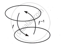
An inverse function takes
us back where we started
Conditions for Invertibility
Properties
-
The inverse of a bijection is also a bijection.
-
The inverse of an inverse function is the original function itself:
\[(f^{-1})^{-1} = f\] -
If you apply a function and then its inverse, you get the original input:
\[f(f^{-1}(x)) = x \quad \text{and} \quad f^{-1}(f(x)) = x\] -
Reversal Law of Inverses: If \[f: A \to B\] and \[g: B \to C\] are both bijections, then their composition \[g \circ f\] is also a bijection, and:
\[(g \circ f)^{-1} = f^{-1} \circ g^{-1}\] -
Reflective Property: The graph of an inverse function \[f^{-1}\] is the exact reflection of the original function f across the diagonal line y = x.
Standard Method to Find an Inverse
To find the inverse of a function:
-
Write \[y = f(x)\].
-
Replace \[f(x)\] by \[y\] and solve for x in terms of y.
-
Interchange x and y.
-
The resulting expression gives \[f^{-1}(x)\], provided the function is invertible.
Definition: Self-Inverse Functions
A Function is called a self-inverse function if its inverse is the exact same as the original function.
-
Condition: \[(f \circ f)(x) = I_x = x\].
-
Examples: \[f(x) = \frac{5}{x}\] and \[g(x) = 7 - x\].
Example 1
Let f : N → Y be a function defined as f(x) = 4x + 3, where,
Y = { y ∈ N : y = 4x + 3 for some x ∈ N }. Show that f is invertible. Find the inverse.
Solution: Consider an arbitrary element y of Y. By the definition of Y, y = 4x + 3, for some x in the domain N. This shows that
\[x=\frac{(y-3)}{4}\]. Define g : Y → N by
\[g(y)=\frac{(y-3)}{4}\]. Now, gof(x) = g(f(x)) = g(4x + 3) = \[\frac{(4x+3-3)}{4}\] = x and
fog(y) = f(g(y)) \[=f\left({\frac{(y-3)}{4}}\right)={\frac{4\left(y-3\right)}{4}}+3\] = y − 3 + 3 = y.
This shows that gof = Iₙ and fog = Iᵧ, which implies that f is invertible and g is the inverse of f.
Example 2
Let f: R → R be defined as f(x) = 10x + 7. Find the function g: R → R such that gof = fog = IR.
Solution:
Step 1: Start from f(x) = 10x + 7
Given f: R → R is defined as f(x) = 10x + 7, for all x ∈ R.
Consider any arbitrary element y of R
As y ∈ R, \[\frac{y-7}{10}\] ∈ R
Step 2: Define g and note its domain, codomain
Let us define g : R → R by g(y) = \[\frac{y-7}{10}\], for all y ∈ R
-
Domain of g = R.
-
Codomain of g = R.
Step 3: Show that gof(x) = x and fog(y) = y
As f: R → R and g: R → R, the composite functions gof and fog both exist.
These can be computed as:
(gof)(x) = g(f(x)) = g(10x + 7)
= \[\frac{(10x+7)-7}{10}\]= x, for all x ∈ R
and (fog)(y) = f(g(y)) = \[\frac{y-7}{10}\] = 10\[\frac{y-7}{10}\] + 7 = y, for all y ∈ R
⇒ gof = fog = IR
Hence, the required function g: R → R is given by
g(y) = \[\frac{y-7}{10}\], for all y ∈ R.
Example 3
If f: R → (−1, 1) is defined by f(x) = \[f(x)=\frac{e^{x}-e^{-x}}{e^{x}+e^{-x}}\] is invertible, find f⁻¹.
Solution:
Let y = f(x), given f is invertible
⇒ \[\frac{e^x-e^{-x}}{e^x+e^{-x}}=\frac{y}{1}\](Apply componendo and dividendo)
⇒ \[\frac{(e^x-e^{-x})+(e^x+e^{-x})}{(e^x-e^{-x})-(e^x+e^{-x})}=\frac{y+1}{y-1}\]
⇒ \[\frac{2e^x}{-2e^{-x}}=\frac{y+1}{y-1}\Rightarrow e^{2x}=\frac{1+y}{1-y}\]
⇒ \[2x=\log_{e}\frac{1+y}{1-y}\Rightarrow x=\frac{1}{2}\log\frac{1+y}{1-y}\]
⇒\[f^{-1}(y)=\frac{1}{2}\log\frac{1+y}{1-y}\]
⇒ f⁻¹(y) = 1/2 logₑ((1 + y)/(1 − y))
Hence,
\[f^{-1}(x)=\frac{1}{2}\log\frac{1+x}{1-x}\]
Example 4
Graph the function and connect the points. Then graph the inverse. Identify the domain and range of each function.
Solution: Switching the x and y values in each ordered pair, the ordered pairs of the inverse functions are obtained as.
| x | 0 | 1 | 2 | 4 | 8 | → | x | 2 | 4 | 5 | 6 | 7 |
| y | 2 | 4 | 5 | 6 | 7 | y | 0 | 1 | 2 | 4 | 8 |
Plotting the points and connecting them, the graph of the given function and its inverse function are obtained as shown in Fig. 2.35. Clearly, the graph of the inverse of the given function is its reflection in the line y = x.
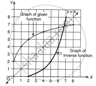
Their domain and range are as follows:
Given function:
Domain : {x : 0 ≤ x ≤ 8}
Range : {y : 2 ≤ y ≤ 7}
Inverse Function:
Domain : {x : 2 ≤ x ≤ 7}
Range : {y : 0 ≤ y ≤ 8}
Key Points: Invertible Functions
- An invertible function is a function that has an inverse.
-
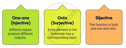
A function is invertible if and only if it is bijective.
-
The graph of \[f^{-1}\] is the reflection of the graph of f in the line y = x.
- \[f^{-1}(f(x)) = x\] and \[f(f^{-1}(x)) = x\]
-
\[(f^{-1})^{-1} = f\]
-
\[(g \circ f)^{-1} = f^{-1} \circ g^{-1}\]
-
An inverse is unique whenever it exists.