Topics
Mathematical Logic
Matrices
Differentiation
Applications of Derivatives
Integration
Definite Integration
Applications of Definite Integration
- Standard Forms of Parabola and Their Shapes
- Ellipse and its Types
- Area Under Simple Curves
- Overview of Application of Definite Integration
Differential Equation and Applications
- Basic Concepts of Differential Equations
- Order and Degree of a Differential Equation
- Formation of Differential Equation by Eliminating Arbitary Constant
- Methods of Solving Differential Equations> Variable Separable Differential Equations
- Methods of Solving Differential Equations> Homogeneous Differential Equations
- Methods of Solving Differential Equations>Linear Differential Equations
- Applications of Differential Equation
- Overview of Differential Equations
Commission, Brokerage and Discount
- Commission and Brokerage Agent
- Concept of Discount
- Overview of Commission, Brokerage and Discount
Insurance and Annuity
- Insurance
- Types of Insurance
- Annuity
- Overview of Insurance and Annuity
Linear Regression
- Regression
- Types of Linear Regression
- Fitting Simple Linear Regression
- The Method of Least Squares
- Lines of Regression of X on Y and Y on X Or Equation of Line of Regression
- Properties of Regression Coefficients
- Overview: Linear Regression
Time Series
- Introduction to Time Series
- Uses of Time Series Analysis
- Components of a Time Series
- Mathematical Models
- Measurement of Secular Trend
- Overview of Time Series
Index Numbers
- Weighted Aggregate Method
- Cost of Living Index Number
- Method of Constructing Cost of Living Index Numbers - Aggregative Expenditure Method
- Overview of Index Numbers
- Method of Constructing Cost of Living Index Numbers - Family Budget Method
- Uses of Cost of Living Index Number
Linear Programming
Assignment Problem and Sequencing
- Assignment Problem
- Hungarian Method of Solving Assignment Problem
- Special Cases of Assignment Problem
- Sequencing Problem
- Types of Sequencing Problem
- Finding an Optimal Sequence
- Overview of Assignment Problem and Sequencing
Probability Distributions
Introduction
In elementary geometry, we learn formulas to calculate the areas of standard geometric figures like triangles, rectangles, trapezoids, and circles. However, these basic formulas fall short when we need to find the area enclosed by arbitrary curves or non-standard shapes.
Finding the area under simple curves, and the area bounded by lines, arcs of circles, parabolas, and ellipses. We do this by visualizing an area as the limit of a sum of infinitesimally thin rectangular strips.
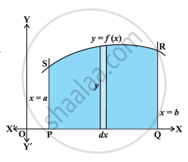
Area Bounded by a Curve and the X-axis
To find the area bounded by the curve y = f(x), the x-axis, and the vertical lines (ordinates) x = a and x = b:
-
Imagine the area as being composed of a very large number of extremely thin vertical strips.
-
Consider an arbitrary elementary strip of height y and width dx.
-
The area of this elementary strip is \[dA = y \cdot dx\].
-
The total area A is the continuous sum (integral) of all these elementary areas from x = a to x = b.
\[A = \int_{a}^{b} y \, dx = \int_{a}^{b} f(x) \, dx\]
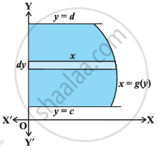
Area Bounded by a Curve and the Y-axis
To find the area bounded by the curve x = g(y), the y-axis, and the horizontal lines y = c and y = d:
-
We consider horizontal strips instead of vertical ones.
-
The elementary strip has length x and infinitesimally small width dy.
-
The area of the strip is \[dA = x \cdot dy\].
\[A = \int_{c}^{d} x \, dy = \int_{c}^{d} g(y) \, dy\]
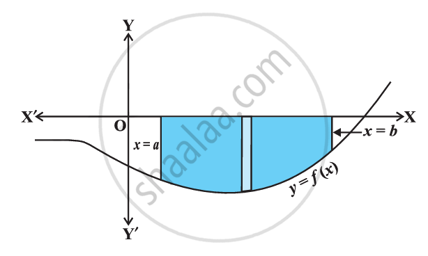
Area Below the X-axis (Negative Area)
If a portion of the curve lies below the x-axis (i.e., f(x) < 0), evaluating the definite integral will yield a negative value. Since physical area cannot be negative, we must take the absolute value (modulus) of the integral.
\[\text{Area} = \left| \int_{a}^{b} f(x) \, dx \right|\]
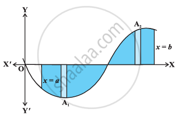
Curve Crossing the X-axis
If a curve crosses the x-axis within the interval [a, b], resulting in area \[A_1\] below the axis and area \[A_2\] above the axis, you cannot integrate from a to $b$ directly (as the negative and positive areas will cancel each other out). The total area is the sum of the absolute values of the separate areas.
\[\text{Total Area } A = |A_1| + A_2\]
Example 1
Find the area enclosed by the ellipse \[\frac{x^2}{a^2} + \frac{y^2}{b^2} = 1\]
Solution:
The area of the region\[ABA'B'A\] bounded by the ellipse
\[= 4 \left( \text{area of the region AOBA in the first quadrant bounded by the curve, } x\text{-axis and the ordinates } x = 0, x = a \right)\]
(as the ellipse is symmetrical about both \[x\]-axis and \[y\]-axis)
\[= 4 \int_{0}^{a} y dx\] (taking vertical strips)
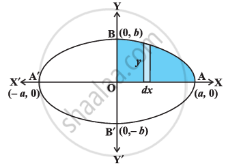
Now \[\frac{x^2}{a^2} + \frac{y^2}{b^2} = 1\] gives \[y = \pm \frac{b}{a} \sqrt{a^2 - x^2}\], but as the region AOBA lies in the first quadrant, \[y\] is taken as positive. So, the required area is
Key Points: Area Under Simple Curves
| Case | Standard Form | Area Formula |
| Region above x-axis | y = f(x) | \[A = \int_{a}^{b} y \, dx\] |
| Region bounded by y-axis | x = g(y) | \[A = \int_{c}^{d} x \, dy\] |
| Curve below x-axis | y = f(x) < 0 | \[A = \left\vert \int_{a}^{b} f(x) \, dx \right\vert\] |
| Curve crossing x-axis | Mixed signs | \[A = \vert A_1 \vert + A_2\] |
