Topics
Demand
- Introduction to Microeconomics and Macroeconomics
- Microeconomics
- Macroeconomics
- Macroeconomics Vs Microeconomics
- Introduction to Demand
- Meaning of Demand
- Features of Demand
- Types of Demand
- Determinants of Demand
- Demand Function
- Quantity Demanded and Demand
- Law of Demand
- Demand Schedule
- Demand Curve
- Individual Demand Curve to Market Demand Curve
- Slope of the Demand Curve
- Linear Demand Curve
- Reasons for the Downward Slope of the Demand Curve
- Importance of the Law of Demand
- Exceptions to the Law of Demand
- Movement Along the Demand Curve
- Change in Demand – Shift in Demand Curve
- Difference Between Extension and Increase in Demand
- Difference Between Contraction and Decrease in Demand
- Cross Price Effects
- Relationship Between Income and Demand
- Impact of Tastes and Preferences on Demand for a Commodity
- Industry Demand Vs Firm Demand
- Concept of Utility
- Cardinal Utility Analysis / Marginal Utility Analysis
- Types of Marginal Utility
- Total Utility and Marginal Utility
- Forms of Utility
- Features of Utility
- Relationship Between Total Utility and Marginal Utility
- Law of Diminishing Marginal Utility
- Exceptions of the Law of Diminishing Marginal Utility
- Importance of the Law of Diminishing Marginal Utility
- Consumer's Equilibrium through Cardinal Utility Approach
- Law of Equi-Marginal Utility
- Exceptions of the Law of Equi-marginal Utility
- Importance of the Law of Equi-marginal Utility
- Ordinal Utility Analysis/Indifference Curve Analysis
- Indifference Schedule
- Indifference Curve
- Indifference Map
- Marginal Rate of Substitution (MRS)
- Assumptions of Indifference Curve Analysis
- Properties of Indifference Curves
- Price Line or Budget Line
- Consumer's Equilibrium through Indifference Curve Approach
- Comparison of Utility Theory and Indifference Curve Theory
- Consumer's Equilibrium through Indifference Curve Approach
- Relationship Between Marginal Rate of Substitution and Marginal Utility
Microeconomic Theory
Theory of Income and Employment
- Introduction to Theory of Income and Employment
- Basic Model of Income Determination
- Aggregate Demand and Its Components
- Desired (Ex Ante) and Effective Demand (Ex Post)
- Propensity to Consume or Consumption Function
- Propensity to Save - Saving Function
- Relationship Between Consumption and Saving Functions
- Derivation of Saving Function
- Investment Expenditure
- Private and Public Investment
- Induced and Autonomous Investment
- Determination of Equilibrium Income and Output
- Concept of Aggregate Demand and Aggregate Supply
- Saving-investment Approach
- Investment Multiplier
- Investment Multiplier Defined
- The Multiplier Mechanism
- Graphic Presentation of Multiplier
- Derivation of Multiplier Formula
- Solved Numerical Problems on Propensity to Consume and Save, Equilibrium Income and Multiplier
- Meaning of Full Employment and Voluntary Unemployment
- The Concept of Full Employment
- Voluntary and Involuntary Unemployment
- Excess Demand
- Measures to Correct the Excess Demand
- Deficient Demand
- Measures to Correct Deficient Demand
- Deficient and Excess Demand and Business Cycle
- Aggregate Demand in a Three - Sector Economy
- Features of the Consumption Function
- Shifting of the Consumption Function
- Importance of the Consumption Function
- Gross Investment and Net Investment
- Paradox of Thrift
- Variables
- Partial and General Equilibrium
- Static Analysis
- Comparative Static Analysis
- Dynamic Analysis
- Difference between Static and Dynamic Analysis
- Psychological Law of Propensity to Consume
- Measures to Raise Propensity to Consume
- Importance of Investment
- Static Multiplier
- Dynamic Concept of Multiplier
- Limitations of Multiplier
- Leakages of Multipler
- Importance of Multiplier
- Types of Multiplier
- Balanced-Budget Multiplier
- Unemployment Associated with Full Employment
- Inflationary Gap
- Foreign Trade Policy
Elasticity of Demand
- Introduction to Elasticity of Demand
- Meaning and Types of Elasticity of Demand
- Price Elasticity of Demand
- Classification of Price Elasticity - Degrees of Price Elasticity of Demand
- Methods of Measuring Price Elasticity of Demand
- Percentage or Proportionate Method
- Total Expenditure Method
- Point Method (Geometric Method)
- Arc Elasticity of Demand
- Revenue Method
- Numerical Problems of Price Elasticity of Demand
- Factors Affecting Price Elasticity of Demand
- Importance of Elasticity of Demand
- Income Elasticity of Demand
- Types of Income Elasticity of Demand
- Importance of Income Elasticity
- Cross Elasticity of Demand
- Туpes of Cross Elasticity of Demand
- Limitations of Cross Elasticity of Demand
- Importance of Cross Elasticity of Demand
Money and Banking
Supply
- Concept of Supply
- Individual and Market Supply
- Distinction Between Supply and Stock
- Determinants of Supply
- Supply Function
- Law of Supply
- Supply Schedule
- Supply Curve
- Derivation of Market Supply Curve From Individual Supply Curves
- Explanation of the Law of Supply
- Time Period and Supply
- Exceptions to the Law of Supply
- Movement Along the Supply Curve Or Expansion and Contraction of Supply
- Shift of the Supply Curve or Change in Supply
- Expansion of Supply and Increase in Supply
- Contraction of Supply and Decrease in Supply
- Elasticity of Supply
- Meaning and Types of Elasticity of Demand
- Price Elasticity of Supply
- Categories (Degrees) of Elasticity of Supply
- Measurement of Elasticity of Supply > Percentage Method
- Measurement of Elasticity of Supply > Geometric or Point Method
- Determinants of Elasticity of Supply
- Importance of Elasticity of Supply
Market Mechanism
- Introduction to Market Mechanism
- Basic Concepts of Equilibrium and Equilibrium Price
- Equilibrium Price and Quantity in a Competitive Market
- Changes in Equilibrium
- Effects of Changes (Shifts) in Demand on Equilibrium Price and Equilibrium Quantity
- Effects of Changes (Shifts) in Supply on Equilibrium Price and Equilibrium Quantity
- Effects of Simultaneous Changes (Shifts) in Demand and Supply
- Some Special Cases of Equilibrium
- Importance of the Element in the Determination of Price
- Applications of Tools of Demand and Supply Price Control
- Mаximum Price Legislation or Price Ceiling and Rationing
- Minimum Price Legislation or Floor Price
- Important Areas of Applications of Tools of Demand and Supply Curves
- Meaning of Perfect Competition
- Assumptions and Conditions of Perfect Competition
- Pure and Perfect Competition
- Time Element in the Theory of Price Determination
- Determination of Equilibrium Prices
- Normal Price and Law of Returns
- Comparison between Market Price and Normal Price
- Practical Applications of Tools of Demand and Supply Analysis
Balance of Payments and Exchange Rate
Public Finance
Concepts of Production
- Concept of Production
- Product
- Factors of Production
- Production Function
- Short-run and Long-run
- Features of Production Function
- Types of Production Functions
- Some Basic Concepts - Total, Average and Marginal Physical Products
- Relationship between Average Product (AP) and Marginal Product (MP)
- Relationship between Total Product (TP) and Marginal Product (MP)
- Returns to a Factor - Laws of Returns to a Variable Factor
- Law of Variable Proportions
- Statement of the Law of Variable Proportions
- Assumptions of the Law of Variable Proportions
- Illustration of the Law of Variable Proportions
- Three Stages of Production
- Explanation of the Law of Variable Proportions
- Stages of Operation and the Decision to Produce
- Conditions Or Causes of Applicability
- Applicability of the Law of Variable Proportions
- Changes in Production
- Returns to a Factor or Law of Returns
- Law of Variable Proportions and Returns to Scale Compared
- Variation of Output in the Long Run - Returns to Scale
- Scale of Production
- Concept of Indivisibility
- Economies of Scale
- Diseconomies of Scale
National Income
Cost and Revenue
- Introduction to Cost of Production
- Money Cost Or Accounting Cost / Explicit Cost
- Economic Cost
- Opportunity Cost
- Real Cost
- Private and Social Cost
- Fixed Cost and Variable Cost
- Different Cost Concepts
- Total Cost Curves
- Average Cost Curves
- Marginal Cost (MC)
- Relationship between Average and Marginal Cost
- Long-Run Cost Curves
- Long-run Average Cost (LAC) Curve
- Long-run Marginal Cost (LMC) Curve
- LAC Curve U-shaped - Economies and Diseconomies of Scale
- Numerical Problems Long-run Cost Curves
- Revenue Concepts
- Behaviour of Revenue Under Different Market Structures
- Relationship Between Total, Average and Marginal Revenues Under Perfect Competition
- Relationship Between Total, Average and Marginal Revenue Under Imperfect Competition
- Significance of Revenue Curve
- Numerical Problems of Revenue
Main Market Forms and Equilibrium of a Firm
- Concept of Market
- Market Structure
- Factors Determining Market Forms
- Perfect Competition
- Features of Perfect Competition
- Pure and Perfect Competition
- Monopoly
- Features of Monopoly
- Monopolistic Competition
- Features of Monopolistic Competition
- Oligopoly
- Features of Oligopoly
- Monopsony
- Features of Monopsony
- Duopoly
- Characteristics of Duopoly
- Bilateral Monopoly
- Other Forms of Market
- Factors Determining Market / Extent of Market
- Demand Curves of Firms under Different Market Forms
- Comparison between different forms of market
- Difference Between Imperfect Competition and Monopolistic Competition
- Firm : An Economic Entity
- Profit Maximisation Objective
- The Definition of Profits
- Rules for Profit-Maximisation
- Producer's (Firm's) Equilibrium: Total Revenue and Total Cost Approach
- Producer's (Firm's) Equilibrium: Marginal Revenue and Marginal Cost Approach
- Short-run Equilibrium
- Long-run Equilibrium
- Firm is a Price Taker, Not a Price Maker
- Equilibrium of Industry
- Difference Between Firm and Industry's Equilibrium
- Meaning of a Producer
- Producer's Equilibrium under Perfect Competition
- Determination of Price and Equilibrium Under Monopoly
- Monopoly Equilibrium and Laws of Costs
- Price Discrimination or Discriminating Monopoly
- Price and Output Discrimination Under Discriminating Monopoly
- Measures of Monopoly Power
- Nature of Demand and Cost Curves
- Equilibrium Price and Output under Monopolistic Competition
- Group Equilibrium in Monopolistic Competition
- Product Differentiation
- Selling Costs
- Equilibrium with Selling Costs
- Price and Output Under Oligopoly Indeterminate
- Price and Output Determination under Oligopoly
- Price Rigidity-Sweezy's Kinky Demand Curve Model or Equilibrium under Independent Action
- Reasons for Price Stability
- Cournot's Model
- Collusive Oligopoly
- Mergers
- Introduction to Static Multiplier
- Forward Working of the Multiplier
- Reverse (Backward) Working of the Multiplier
- Saving-Investment Equality Approach
- Key Points: Static Multiplier
Introduction to Static Multiplier
In the static multiplier, there is no time lag between the original and the new equilibrium. The increase in investment leads to an increase in income in the same period. All economic variables — investment, income, and consumption — are related to the same period. The time interval between the two equilibria (known as the generation period) is not considered.
Gardner Ackley described this as a "fixed period analysis" — it compares the starting equilibrium with the final equilibrium without tracking what happens in between.
Prof. Samuelson's Warning
The multiplier is a two-edged sword. It will cut for you or go against you." — This means the multiplier works both in forward and backward directions, i.e., to raise or reduce income.
Forward Working of the Multiplier
The forward working of the multiplier states that an increase in investment leads to a multiplied increase in the level of income.
Multiplier Table (MPC = 0.5)
| Round | ΔI (Investment) | ΔY (Income) | ΔC (Consumption) | ΔS (Saving) |
|---|---|---|---|---|
| 1 | ₹200 Cr | ₹200 Cr | ₹100 Cr | ₹100 Cr |
| 2 | — | ₹100 Cr | ₹50 Cr | ₹50 Cr |
| 3 | — | ₹50 Cr | ₹25 Cr | ₹25 Cr |
| 4 | — | ₹25 Cr | ₹12.50 Cr | ₹12.50 Cr |
| 5 | — | ₹12.50 Cr | ₹6.25 Cr | ₹6.25 Cr |
| 6 | — | ₹6.25 Cr | ₹3.12 Cr | ₹3.12 Cr |
| Total | ₹200 Cr | ₹400 Cr | ₹200 Cr | ₹200 Cr |
Mathematical Derivation
ΔY = ΔI × (1 + c + c² + c³ + …) = ΔI / (1 − c)
Substituting: ΔY = 200 / (1 − 0.5) = 200 / 0.5 = ₹400 crores
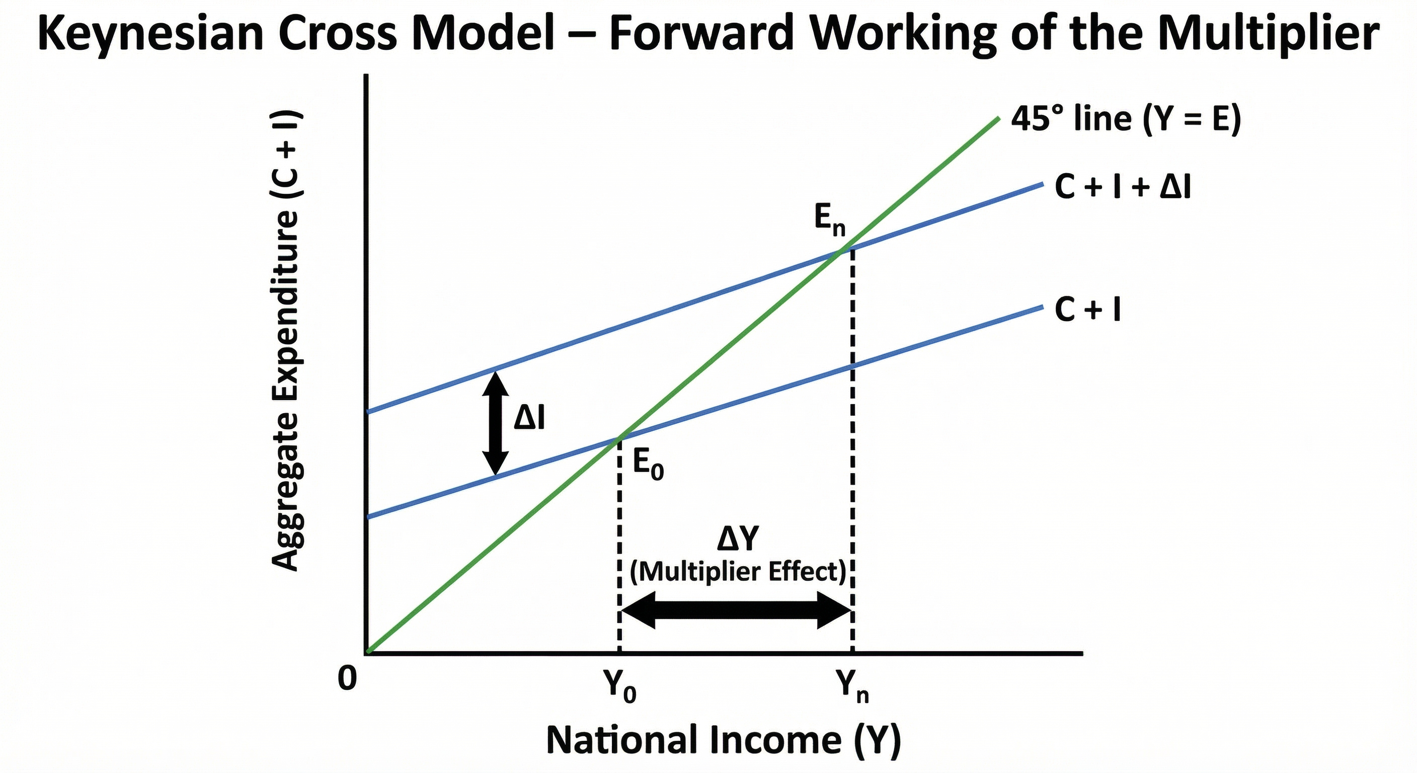
Keynesian Cross Diagram (AD-AS Approach)
How to Read This Diagram
- Axes: X-axis = National Income (Y); Y-axis = Aggregate Expenditure (C + I). The 45° line shows where Income = Expenditure (equilibrium condition).
- Original Equilibrium: C + I line intersects the 45° line at point E₀ → Equilibrium income = OY₀. At this point, OY₀ = E₀Y₀.
- Investment Increases: When investment rises by ΔI, expenditure line shifts upward to C + I + ΔI.
- New Equilibrium: New expenditure line intersects 45° line at Eₙ → New income = OYₙ.
- Multiplier Effect: The increase from OY₀ to OYₙ is greater than ΔI. This is the forward multiplier effect.
Reverse (Backward) Working of the Multiplier
Just as an increase in investment causes a multiplied rise in income, a decrease in investment causes a multiplied fall in income.
How Reverse Multiplier Works
- Starting from equilibrium at Eₙ where income = OYₙ.
- Investment falls → Expenditure line shifts downward from C + I + ΔI back to C + I.
- Equilibrium shifts back to E₀ → Income falls from OYₙ to OY₀.
- The fall in income is a multiple of the fall in investment.
If investment falls by ₹200 Cr and MPC = 0.5 (K = 2), then income falls by ₹200 × 2 = ₹400 Cr.
Saving-Investment Equality Approach
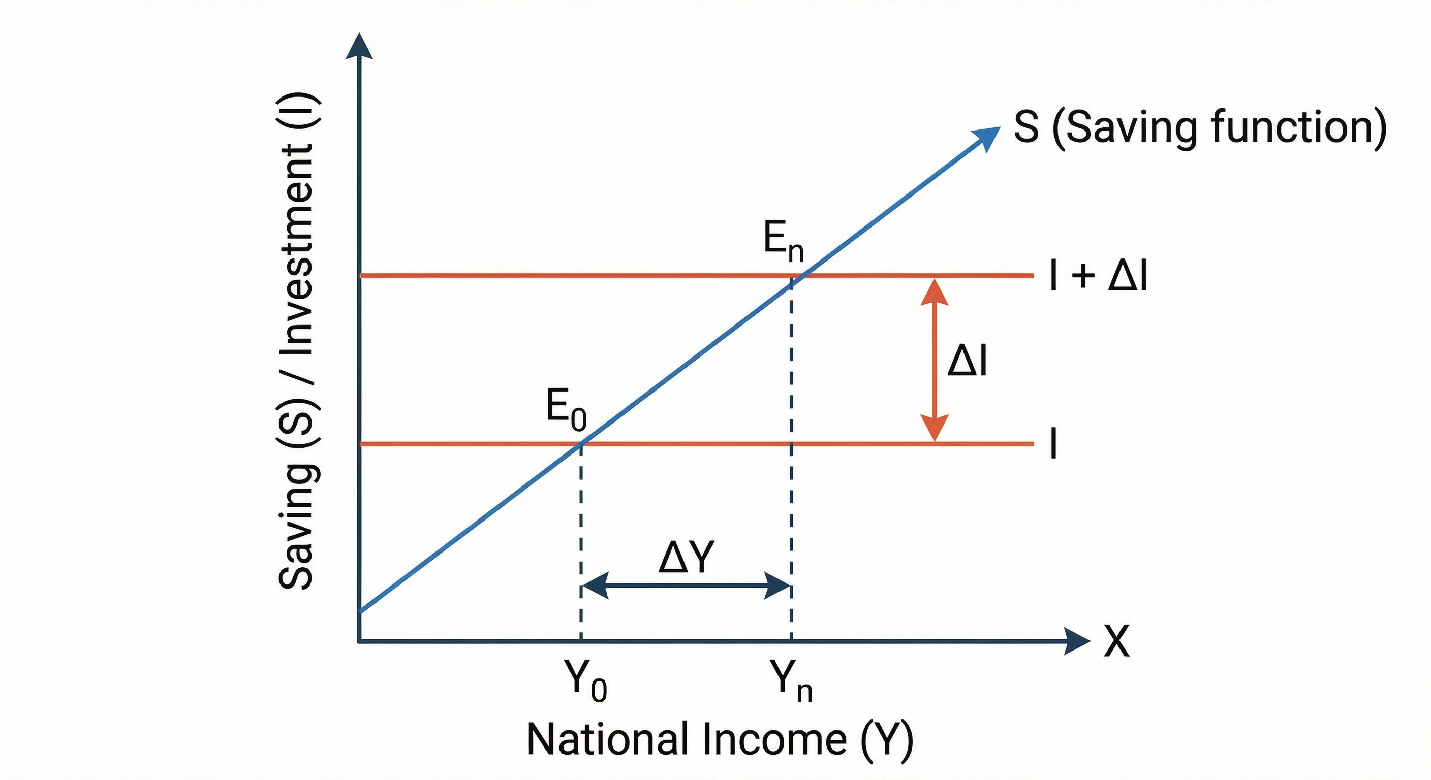
This is an alternative method to demonstrate the multiplier, using the condition that equilibrium occurs where Saving = Investment.
How to Read This Diagram
- X-axis: National Income (Y); Y-axis: Saving (S) & Investment (I)
- S-curve (Saving function): Upward sloping — savings increase with income. This is an induced function.
- I-line (Investment): Horizontal — autonomous investment that does not depend on income (e.g., government welfare spending).
Key Points: Static Multiplier
- In a static multiplier, there is no time lag; increase in investment raises income in the same period.
- All variables (income, consumption, investment) belong to the same time period.
- Multiplier works in two directions:
Forward: Increase in investment → multiple increase in income.
Reverse: Decrease in investment → multiple fall in income. - Size of income change depends on MPC and saving–investment equality.
