Revision: Microeconomic Theory >> Laws of Returns: Returns to a Factor and Returns to Scale Economics ISC (Commerce) Class 12 CISCE

Older definitions: Production is making material goods.
Newer (economic) definitions: Production is creating value for sale or paid services.

• Fraser: “Production means—putting utility into.”
• Cairncross: “Making goods for sale or rendering paid services.”
• Meyers: “Any activity resulting in goods/services meant for exchange.”

Capital consists of all those goods, existing at present time which can be used in anyway, so as to satisfy wants during the subsequent years.

Production means creation of 'material goods' only. For example, if a farmer is growing wheat, we will say the farmer is producing wheat. Likewise, if a carpenter is making a table, it will be said that the carpenter is producing table. Adam Smith, 'the Father of Economics', has defined production in this sense. According to him, "Production means production of material goods only."

A production function indicates the highest amount of a product that can be made in a specific time frame using a set amount of inputs, utilising the best available production method.

A production function shows the maximum quantity of a commodity that can be produced per unit of time with the given amount of inputs when the best production technique available is used. A production function can be expressed in the form of a table, graph or algebraic equation. In the form of an algebraic equation, the production function for a good may be expressed as:

Q_X = f(F₁, F₂...F_n) Where O_X is the quantity of output of the commodity X: and  F₁, F₂ ... F_n are the quantities of different inputs used to produce the commodity X.

Total quantity of output produced by using given units of a variable input (like number of workers) with fixed inputs.

Extra output produced when one more unit of a variable input is used, keeping other inputs fixed.

• "The term returns to scale refers to the changes in output as all factors change by the same proportion." — Koutsoyiannis
• "Returns to scale relates to the behaviour of total output as all inputs are varied and is a long run concept." — Leibhafsky

• “As the proportion of the factor in a combination of factors is increased after a point, first the marginal and then the average product of that factor will diminish.”
  —Benham
• “The law of variable proportion states that if the inputs of one resource is increased by equal increment per unit of time while the inputs of other resources are held constant, total output will increase, but beyond some point the resulting output increases will become smaller and smaller.”
  —Leftwich
• “An increase in some inputs relative to other fixed inputs will, in a given state of technology, cause output to increase; but after a point the extra output resulting from the same additions of extra inputs will become less and less.”
  —Samuelson

A production function can be shown as:

• A table (showing different combinations of inputs and output),
• A graph, or
• An equation (algebraic form).

General form:

\[Q_x=f(f_1,f_2,\ldots,f_n)\]

Where:

• Q_x = quantity of output of commodity X,
• f₁, f₂,…, f_n = quantities of different factor inputs,
• Q_x is the dependent variable (depends on inputs) ,
• f₁, f₂,…, f_n are independent variables.

If we assume only two inputs: labour (L) and capital (K):

\[Q_x=f(L,K)\]

The law of variable proportions (LVP) states that as we increase the quantity of only one input, keeping other inputs fixed, total product (TP) initially increases at an increasing rate, then at a decreasing rate and finally at a negative rate.

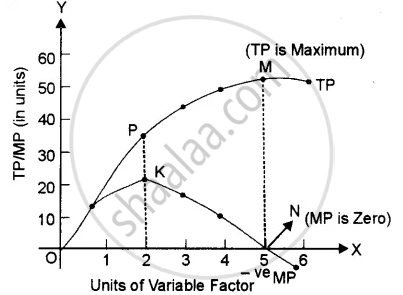
In the given diagram, the quantity of the variable factor has been measured on X-axis and the Y-axis measures the total product on the Y-axis. The diagram indicates how the total product and marginal product change as a result of increases in the quantity of one factor to a fixed quantity of other factors.

The law can be better explained through three stages:

1. First stage:
   • Increasing return to a factor: In the first stage, every additional variable factor adds more and more to the total output. It means TP increases at an increasing rate and the MP of each variable factor rises. Better utilisation of fixed factors and increases in the efficiency of a variable factor due to specialisation are the major factors responsible for increasing returns. The increasing returns to a factor stage have been shown in the given diagram between O to P. It implies. TP increases at an increasing rate (till point ‘P’) and MP rises till it reaches its maximum point ‘K,’ which marks the end of the first phase.
     
2. Second stage:
   • Diminishing returns to a Factor: In the second stage, every additional variable factor adds a lesser and lesser amount of output. It means TP increases at a diminishing rate and MP falls with an increase in a variable factor. The breaking of the optimum combination of a fixed and variable factor is the major factor responsible for diminishing returns. The second stage ends at point ‘S’ when MP is zero and TP is maximum (point ‘M’).
     Stage 2 is very crucial, as a rational producer will always aim to produce in this phase because TP is maximum and MP of each variable factor is positive.
3. Third stage:
   • Negative Returns to a Factor: In the third stage the employment of additional variable factors causes TP to decline. MP now becomes negative. Therefore, this stage is known as negative returns to a factor. Poor coordination between variable and fixed factors is the basic cause for this stage. In the fig., the third stage starts after point ‘N’ on the MP curve and point ‘O’ on the TP curve. The MP of each variable factor is negative in the 3 stages. So, no firm would deliberately choose to operate in this stage.

• If you keep increasing the variable input (e.g., labour) for a fixed input (e.g., land), the total production goes up at first, then grows slowly, and finally can go down.
• Marginal product (extra output from one more unit) and average product (output per unit) also rise at first, but later start to fall.

• Production is any process that adds value/utility for sale or exchange.
• All four factors (land, labour, capital, and organisation) must be balanced.
• Efficiency is when each factor’s extra contribution matches its cost.
• Services and goods are both considered production.

• Products include both goods and services, and both satisfy human wants.
• Goods are tangible, services are intangible.
• On the basis of productive activities, products are primary, secondary, or tertiary.
• On the basis of process of production, products are intermediate (inputs) or final (ready for use).
• On the basis of durability, goods are non-durable (short life) or durable (long life).
• On the basis of use, products are consumer goods (for direct consumption) or investment/capital goods (for further production).
• The same good can be consumer or investment good, depending on how it is used.

• Four main factors: Land, Labour, capital, and Entrepreneurship.
• All production needs these factors.
• Each factor works together to create goods/services.

• A production function shows the technical relationship between physical inputs and maximum possible output in a given time.
• Short run: At least one factor is fixed; the firm changes output by changing only variable factors.
• Long run: All factors are variable; the firm can change the scale of production and plant size.
• Short‑run production function Q = f (L) → study of returns to a factor and Law of Variable Proportions.
• Long‑run production function Q = f (K, L) → study of returns to scale.

• TP increases first, gets maximum, then may fall.
• AP is average for each worker; it first rises, then falls.
• MP is the extra that comes from each new worker; it rises, then falls, and can become negative.

• AP = output per unit of variable factor; MP = extra output from one more unit.​
• When MP > AP, AP rises; when MP = AP, AP is maximum; when MP < AP, AP falls.​
• The MP curve cuts the AP curve at the maximum point of AP.​
• MP can be positive, zero, or negative; AP stays positive as long as output is positive.​
• The AP–MP relationship follows the general “marginal vs average” rule used in many areas of economics.

• TP = total output; MP = extra output from one extra unit of input.
• MP is the rate of change (slope) of TP.
• Rising MP → TP rises faster (increasing rate).
• Falling but positive MP → TP still rises but more slowly (diminishing rate).
• MP = 0 → TP at its maximum level.
• MP negative → TP falls as more input is added.

• Only one input is changed; others are fixed.
• First, output improves quickly.
• Later, output slows down and may decrease.
• Businesses use this law to find the best input mix.

• Law of Variable Proportions: Output rises at first, then slower, then falls when adding more of one input to fixed resources.
• Three stages: Increasing, Diminishing, and Negative Returns.
• Practical example: Adding more workers to a set number of machines.

• Law of variable proportions is a short‑run law explaining how output changes when one input varies and others are fixed.​
• There are three stages: Stage I (increasing returns), Stage II (diminishing returns), Stage III (negative returns).​
• Stages I and III are “non‑economic” regions; Stage II is the only rational region for a producer.
• A rational producer always operates in Stage II; the exact point depends on input and output prices.​
• The law applies to agriculture, industry, and any production where at least one factor is fixed in the short run.

• In the long run, all factors are variable and the firm can change its scale of production.
• Returns to scale describe how output changes when all inputs are increased in the same proportion.​
• There are three types:
  (i) Increasing returns to scale – output increases more than proportionately.
  (ii) Constant returns to scale – output increases in the same proportion.
  (iii) Decreasing returns to scale – output increases less than proportionately.​
• Internal economies (specialisation, better organisation) lead to increasing returns to scale, while internal diseconomies (coordination and management problems) lead to decreasing returns to scale.​

• Law of Variable Proportions: Studies change in one factor; short-run; input mix changes.
• Returns to Scale: Studies change in all factors together; long-run; input proportions remain constant.

• Scale of production refers to firm output size.
• It depends on technology and market demand.
• Indivisibility means some inputs force firms to produce at larger scales for cost efficiency.

• Economies of scale help firms reduce average costs as production increases.
• Internal economies include technical, marketing, labour, managerial, and transport/storage economies plus pecuniary savings.
• External economies come from industry growth and infrastructure shared by all firms.
• Understanding these helps firms and policymakers improve production efficiency.

• Diseconomies of scale increase costs when a firm grows too big.
• Internal diseconomies arise from management, technical, production, marketing, and financial issues.
• External diseconomies come from pollution, infrastructure overload, and resource competition.
• Understanding these helps firms stay efficient and avoid costly expansion.

• Economies reduce costs; diseconomies increase costs in expanding industries.
• The balance between these decides the industry's cost dynamics and classification.