Definitions [11]
According to Hicks, "It is the locus of the points representing parts of quantities between which the individual is indifferent and so it is termed as an indifference curve."
According to Meyres, "An indifference curve may be defined as a schedule of various combinations of goods which will be equally satisfactory to the consumer concerned."
According to Ferguson, "An indifference curve is a combination of goods, each of which yields the same level of total utility for which the consumer is indifferent." According to Leftwich, "A single indifference curve shows the different combinations of X and Y that yield equal satisfaction to the consumer."
- "Want is effective desire for particular thing which expresses itself in the effort or sacrifice necessary to obtain them." – Peterson
- "The demand for anything at a given price is the amount of it which will be bought per unit of time at that price." – Prof. Benham
- "By demand, we mean the quantity of a commodity that will be purchased at a particular price and not merely the desire of a thing." – Hansen
- "The demand for a particular good is the amount that will be purchased at a given price and at a given time." – Veera Anstey
Define the following concept:
Derived demand
When goods are demanded so that they can be used in the production of some other commodity, it is called indirect or derived demand.
Define the concept of demand schedule.
A tabular representation that shows the quantity of a good a consumer is willing to purchase at different prices, over a specific period of time.
Define individual demand.
Individual demand refers to the quantity of the commodity that an individual household is willing to buy at different prices in a given period of time.
Define price elasticity of demand.
It is the measure of the degree of responsiveness of the demand for a good to the changes in its price. It is defined as the percentage change in the demand for a good divided by the percentage change in its price.
ed = `"Percentage change in demand for good"/"Percentage change in price of that good"`
ed = `(ΔQ)/(ΔP) xx P/Q`
Where ΔQ = Q2 − Q1, change in demand
ΔP = P2 − P1, change in price
P1 = Initial price
Q1 = Initial quantity
Define elasticity of demand.
Price elasticity of demand tells us the amount of the change in the quantity demanded of a commodity in response to change in its price. In other words, it measures the degree of change of demand in response to changes in price.
Define the following concept:
Cross Elasticity of Demand
Cross elasticity of demand is the measure of the responsiveness of demand for a good to a change in the price of a related good.
`"Ec" = ("Proportionate change in quantity demanded of good X")/("Proportionate change in price of good Y")`
- "Elasticity of demand may be defined as the percentage change in quantity demanded to the percentage change in price." - Alfred Marshall
- "The elasticity of demand for a commodity is the rate at which quantity bought changes as the price changes." - A.K. Cairncross
- "Elasticity of demand is a technical term used by the economists to describe the degree of respensiveness of demand of a commodity to a change in its price." -Stonier and Hague
- Elasticity of demand refers to the degree of responsiveness of quantity demanded of a commodity to a change in any of its determinants.
- "Income elasticity of demand means the ratio of the percentage change in the quantity demanded to the percentage change in income." - Watson
- "The responsiveness of demand to change in income is termed as income elasticity of demand." - R.G. Lipsey
Formulae [2]
Demand = Desire + Willingness to Buy + Ability to Pay
Ey = `"Proportionate change in Quantity Demanded"/"Proportionate change in income"`
\[E_y=\frac{\frac{\Delta Q}{Q}}{\frac{\Delta Y}{Y}}\quad=\frac{\Delta Q}{Q}\div\frac{\Delta Y}{Y}=\frac{\Delta Q}{Q}\times\frac{Y}{\Delta Y}\]
Where:
Ey = Income elasticity of demand
ΔQ = Change in the quantity demanded
Q = Initial demand
ΔY = Change in income
Y = Initial Income
Theorems and Laws [2]
State and explain the law of demand.
The law of demand was introduced by Prof. Alfred Marshall in his book, ‘Principles of Economics’, which was published in 1890. The law explains the functional relationship between price and quantity demanded.
According to Prof. Alfred Marshall, “Other things being equal, the higher the price of a commodity, the smaller is the quantity demanded, and the lower the price of a commodity, the larger is the quantity demanded.” In other words, other factors remaining constant, if the price of a commodity rises, demand for it falls; and when the price of a commodity falls, demand for it rises. Thus, there is an inverse relationship between price and quantity demanded. Symbolically, the functional relationship between demand and price is expressed as:
Dx = f (Px)
Where D = Demand for a commodity
x = Commodity
f = Function
Px = Price of a commodity
| Price of a commodity ‘x’ (₹) |
Quantity demanded of the commodity ‘x’ (in kgs.) |
| 50 | 1 |
| 40 | 2 |
| 30 | 3 |
| 20 | 4 |
| 10 | 5 |
As shown in the table, when the price of commodity ‘x’ is ₹ 50, the quantity demanded is 1 kg. When the price falls from ₹ 50 to ₹ 40, the quantity demanded rises from 1 kg to 2 kg. Similarly, at a price of ₹ 30, the quantity demanded is 3 kgs, and when the price falls from ₹ 20 to ₹ 10, the quantity demanded rises from 4 kgs to 5 kgs. Thus, as the price of a commodity falls, quantity demanded rises, and when the price of the commodity rises, quantity demanded falls. This shows an inverse relationship between price and quantity demanded.

The X-axis represents the demand for the commodity, and the Y-axis represents the price of the commodity x. DD is the demand curve, which slopes downward from left to right because price and quantity demanded are inversely related.
State and explain the ‘law of demand’ with its exceptions.
Prof. Alfred Marshall introduced the law of demand in his book, ‘Principles of Economics,’ published in 1890. The law explains the functional relationship between price and quantity demanded.
- Statement of the Law: According to Prof. Alfred Marshall, “Other things being equal, the higher the price of a commodity, the smaller the quantity demanded, and the lower the price of a commodity, the larger the quantity demanded.” Explanation: Other factors remain constant: when the price of a commodity rises, demand for it falls, and when the price of a commodity falls, demand for it rises. Thus, there is an inverse relationship between price and quantity demanded.
- Demand Schedule: The law of demand is explained with the help of the following demand schedule:
Demand Schedule Price of commodity
‘x’ (in ₹)Quantity demanded
per week (in kg)10 1 8 2 6 3 4 4 2 5 - From the above schedule, it can be observed that when the price of the commodity is ₹ 10, the demand is 1 kg.
- When the price falls from ₹ 10 to ₹ 8, the demand rises from 1 kg to 2 kg.
- Similarly, as the price falls from ₹ 8 to 6 and from ₹ 6 to 4, the demand rises from 2 kg to 3 kg and 3 kg to 4 kg, respectively.
- If we look at the schedule from bottom to top, when the price rises from ₹ 2 to ₹ 4, the demand falls from 5 kg to 4 kg.
- Thus, we can conclude that as the price of a commodity falls, the quantity demanded rises, and when the price of the commodity rises, the quantity in demand falls.
- This shows an inverse relationship between price and quantity demanded.
- Demand Curve: The law of demand can be further explained with the help of the following demand curve:

In the above diagram, the Y-axis represents price, and the X-axis represents quantity demanded. DD is the demand curve that slopes downward from left to right. It represents the inverse relation between price and quantity in demand. - Exceptions: The exceptions to the law are as follows:
- Giffen’s paradox: Giffen Goods are inferior or low-quality goods like vanaspati ghee (Dalda), low-quality rice, etc. These are goods whose demand does not rise, even if their price falls. This happens because every person wants to increase their standard of living constantly.
Sir Robert Giffen observed this behaviour related to bread (an inferior good) in England. People had limited money, so they consumed more bread (a cheaper commodity) and less meat (a costlier commodity). He observed that when the price of bread decreased, less bread was demanded than before. The people saved money and used it to purchase meat, and thus, the demand for meat increased. This behaviour is called “Giffen’s paradox”. There is a direct relationship between price and quantity demanded in the case of Giffen goods. The demand curve for Giffen goods slopes upward from left to right. - Speculation: The law of demand does not hold true when people expect prices to rise further. In this case, although prices have risen today, consumers will demand more in anticipation of a further rise in the price. For example, during the epic lockdown in March 2020, people expected the prices of goods to rise in the future. Therefore, they purchased goods in large quantities, even at high prices.
- Habitual Goods: If a person is habituated to or addicted to certain goods, his demand for these goods will continue to be the same even if the price of such goods rises. For example, people addicted to social media like FB, TikTok, Instagram, etc., will not reduce their usage even if the data packs or internet usage rates are increased.
- Illusion of Price: Consumers may believe that high-priced goods are of better quality; therefore, demand for such goods tends to increase with an increase in their prices. For example, expensive branded products are in demand, even at high prices.
- Prestige Goods: Prestige goods are regarded as a status symbol in society. Rich people may demand more of these goods when their prices rise to show off. E.g. Gold, diamonds, expensive watches, luxury cars, etc.
- Fashion: A product that is out of fashion (e.g., keypad phones) will have less demand even if the price falls. A product in fashion (e.g., smartphones) will have a high demand even if the price rises. Thus, it is an exception to the law.
- Ignorance: Sometimes, people buy more of a commodity at high prices due to ignorance. This may happen because the consumer is not aware of the cost of the commodity at other places.
- Necessities: The demand for specific necessities like basic foodstuffs (wheat, salt, dal, etc.) will not change due to a change in their prices.
- Demonstration Effect: The tendency of the low-income group to imitate the consumption pattern of high-income groups is known as the demonstration effect. For example, the T-shirts “Being Human” by Salman Khan are in very high demand despite their high prices.
- Giffen’s paradox: Giffen Goods are inferior or low-quality goods like vanaspati ghee (Dalda), low-quality rice, etc. These are goods whose demand does not rise, even if their price falls. This happens because every person wants to increase their standard of living constantly.
Introduction: The law of demand was introduced by Prof. Alfred Marshall in his book ‘Principles of Economics’, published in 1890. The law explains the functional relationship between price and quantity demanded.
Statement of the Law: According to Prof. Alfred Marshall, “Other things being equal, higher the price of a commodity, smaller is the quantity demanded and lower the price of a commodity, larger is the quantity demanded.”
In other words, other factors remaining constant, if the price of a commodity rises, demand for it falls and when price of a commodity falls demand for the commodity rises. Thus, there is an inverse relationship between price and quantity demanded.
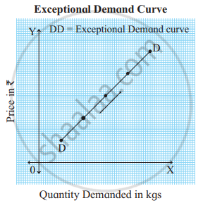
Exceptions to the Law of Demand: There are certain exceptions to the law of demand. It means that under exceptional circumstances, consumer buys more when the price of commodity rises and buys less when price of commodity falls. In such cases, demand curve slopes upwards from left to right. i.e. the demand curve has a positive slope as shown in figure.
Following are the exceptions to the law of demand:
- Giffen’s paradox: Inferior goods or low-quality goods are those goods whose demand does not rise even if their price falls. At times, demand decreases when the price of such commodities falls. Sir Robert Giffen observed this behaviour in England regarding bread. He noted that, when the price of bread declined, people did not buy more because of an increase in their real income or purchasing power. They preferred to buy superior goods like meat. This is known as Giffen’s paradox.
- Prestige goods: Expensive goods like diamonds, gold, etc., are status symbols. So rich people buy more of it, even when their prices are high.
- Speculation: The law of demand does not hold true when people expect prices to rise still further. In this case, although prices have risen today, consumers will demand more in anticipation of a further price rise. For example, prices of oil, sugar, etc., tend to rise before Diwali. So people continue purchasing more at high prices, anticipating that prices may rise during Diwali.
- Price illusion: Consumers believe that high-priced goods are of better quality. Therefore, the demand for such goods tends to increase with a rise in their prices. For example, expensive branded products are in demand even at high prices.
- Ignorance: Sometimes, due to ignorance, people buy more of a commodity at a high price. This may happen when consumer is ignorant about the price of that commodity at other places.
- Habitual goods: Due to habitual consumption, certain goods, such as tea, are purchased in required quantities even at higher prices.
Key Points
- Micro demand = individual level; macro demand = whole economy (aggregate) level.
- Both levels must mention price and time for demand to make sense.
- Demand is always a “flow” concept—measured as so much per time period.
- Demand is affected by many factors, not just price.
- A change in any determinant—like income, preferences, or population—can shift demand.
- Some factors (like climate or government taxes) have seasonal or policy-based effects.
- Related goods can be substitutes (used instead) or complements (used with).
- Real-life decisions—like bulk buying before a GST rise—are practical examples of demand determinants at work.
- A demand schedule helps predict the quantity consumers will buy at different prices.
- It demonstrates the law of demand: as price falls, demand increases.
- The demand curve is the graphical version of the demand schedule, always sloping downwards.
- Both individual and market schedules are useful for setting prices, planning production, and understanding consumer behaviour.
- The demand curve represents the law of demand visually.
- There are two types: individual and market demand curves.
- The market demand curve is derived by summing individual curves at each price.
- Movements along the curve are due to price changes; curve shifts are due to outside factors.
- Law of demand only shows direction (more or less), elasticity shows the degree (how much more or less).
- Some things (necessities) have inelastic demand; luxuries or goods with many substitutes have elastic demand.
- Alfred Marshall introduced this concept and the popular measurement formula.
- YED shows how demand changes with income.
- Luxury goods: YED > 1 → demand grows faster than income.
- Necessities: 0 < YED < 1 → demand grows slower than income.
- Essential goods: YED = 0 → demand stays the same.
- Inferior goods: YED < 0 → demand drops as income rises.
- Total Expenditure Formula:
Total Expenditure (TE) = Price (P) × Quantity Demanded (Q) - Revenue Method Formula:
Ed = AR / (AR - MR)
or
Ed = Average Revenue / (Average Revenue - Marginal Revenue) - Arc Elasticity Demand Formula:
\[\mathrm{E=\frac{Q_{2}-Q_{1}}{Q_{2}+Q_{1}}\div\frac{P_{1}-P_{2}}{P_{1}+P_{2}}}\] - Proportionate Method Formula:
\[\mathrm{Ed}=\frac{\text{Percentage change in Quantity demanded}}{\text{Percentage change in Price}}\]
\[\mathrm{Ed}=\frac{\%\triangle\mathrm{Q}}{\%\triangle\mathrm{P}}\]
Concepts [12]
- Consumer's Equilibrium
- Cardinal Approach (Utility Analysis)
- Ordinal Utility Analysis/Indifference Curve Analysis
- Concept of Demand
- Market Demand
- Determinants of Demand
- Demand Schedule
- Demand Curve
- Movement along the Demand Curve and Shift of the Demand Curve
- Concept of Elasticity of Demand
- Types of Elasticity of Demand > Income Elasticity
- Methods of Measuring Price Elasticity of Demand
