Advertisements
Advertisements
प्रश्न
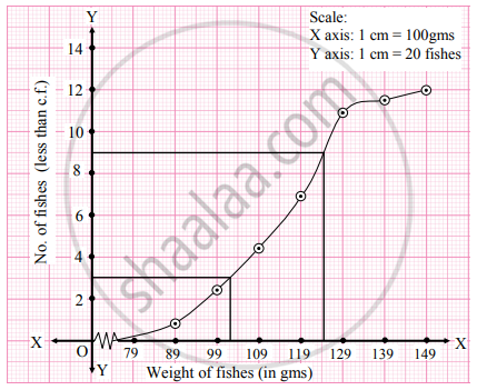
Draw ogive for the Following distribution and hence find graphically the limits of weight of middle 50% fishes.
| Weight of fishes (in gms) | 800 – 890 | 900 – 990 | 1000 – 1090 | 1100 – 1190 | 1200 – 1290 | 1300 –1390 | 1400 – 1490 |
| No. of fishes | 8 | 16 | 20 | 25 | 40 | 6 | 5 |
Advertisements
उत्तर
Since the given data is not continuous, we have to convert it in the continuous form by subtracting 5 from the lower limit and adding 5 to the upper limit of every class interval. To draw a ogive curve, we construct the less than cumulative frequency table as given below:
| Weight of fishes (in gms) |
No. of fishes (f) |
Less than cumulative frequency (c.f.) |
| 795 – 895 | 8 | 8 |
| 895 – 995 | 16 | 24 |
| 995 – 1095 | 20 | 44 |
| 1095 – 1195 | 25 | 69 |
| 1195 – 1295 | 40 | 109 |
| 1295 – 1395 | 6 | 115 |
| 1395 – 1496 | 5 | 120 |
| Total | 120 |
Points to be plotted are (895, 8), (995, 24),(1095, 44),(1195, 69),(1295, 109), (1395, 115), (1495, 120).
N = 120
For Q1 and Q3 we have to consider `"N"/4=120/4` = 30, `(3"N")/4=(3xx120)/4` = 90
For finding Q1 and Q3 we consider the values 30 and 90 on the Y-axis. From these points, we draw the lines which are parallel to X-axis. From the points where these lines intersect the less than ogive, we draw perpendicular on X-axis. The feet of perpendiculars represent the values of Q1 and Q2.
∴ Q1 ≈ 1025 and Q3 ≈ 1248
∴ The limits of weight of middle 50% fishes lie between 1025 to 1248.
APPEARS IN
संबंधित प्रश्न
The following table gives frequency distribution of marks of 100 students in an examination.
| Marks | 15 –20 | 20 – 25 | 25 – 30 | 30 –35 | 35 – 40 | 40 – 45 | 45 – 50 |
| No. of students | 9 | 12 | 23 | 31 | 10 | 8 | 7 |
Determine D6, Q1, and P85 graphically.
The following table gives the distribution of daily wages of 500 families in a certain city.
| Daily wages | No. of families |
| Below 100 | 50 |
| 100 – 200 | 150 |
| 200 – 300 | 180 |
| 300 – 400 | 50 |
| 400 – 500 | 40 |
| 500 – 600 | 20 |
| 600 above | 10 |
Draw a ‘less than’ ogive for the above data. Determine the median income and obtain the limits of income of central 50% of the families.
The following frequency distribution shows the profit (in ₹) of shops in a particular area of city:
| Profit per shop (in ‘000) | No. of shops |
| 0 – 10 | 12 |
| 10 – 20 | 18 |
| 20 – 30 | 27 |
| 30 – 40 | 20 |
| 40 – 50 | 17 |
| 50 – 60 | 6 |
Find graphically The limits of middle 40% shops.
The following frequency distribution shows the profit (in ₹) of shops in a particular area of city:
| Profit per shop (in ‘000) | No. of shops |
| 0 – 10 | 12 |
| 10 – 20 | 18 |
| 20 – 30 | 27 |
| 30 – 40 | 20 |
| 40 – 50 | 17 |
| 50 – 60 | 6 |
Find graphically the number of shops having profile less than 35,000 rupees.
The following is the frequency distribution of overtime (per week) performed by various workers from a certain company.
Determine the values of D2, Q2, and P61 graphically.
| Overtime (in hours) |
Below 8 | 8 – 12 | 12 – 16 | 16 – 20 | 20 – 24 | 24 and above |
| No. of workers | 4 | 8 | 16 | 18 | 20 | 14 |
Draw ogive for the following data and hence find the values of D1, Q1, P40.
| Marks less than | 10 | 20 | 30 | 40 | 50 | 60 | 70 | 80 | 90 |
| No. of students | 4 | 6 | 24 | 46 | 67 | 86 | 96 | 99 | 100 |
The following table gives the distribution of females in an Indian village. Determine the median age of graphically.
| Age group | No. of females (in ‘000) |
| 0 – 10 | 175 |
| 10 – 20 | 100 |
| 20 – 30 | 68 |
| 30 – 40 | 48 |
| 40 – 50 | 25 |
| 50 – 60 | 50 |
| 60 – 70 | 23 |
| 70 – 80 | 8 |
| 80 – 90 | 2 |
| 90 – 100 | 1 |
Find graphically the values of D3 and P65 for the data given below:
| I.Q of students | 60 – 69 | 70 – 79 | 80 – 89 | 90 – 99 | 100 – 109 | 110 – 119 | 120 – 129 |
| No. of students | 20 | 40 | 50 | 50 | 20 | 10 | 10 |
Determine graphically the value of median, D3, and P35 for the data given below:
| Class | 10 – 15 | 15 – 20 | 20 – 25 | 25 – 30 | 30 – 35 | 35 – 40 | 40 – 45 |
| Frequency | 8 | 14 | 8 | 25 | 15 | 14 | 6 |
Draw an ogive for the following distribution. Determine the median graphically and verify your result by mathematical formula.
| Height (in cms.) | No. of students |
| 145 − 150 | 2 |
| 150 − 155 | 5 |
| 155 − 160 | 9 |
| 160 − 165 | 15 |
| 165 − 170 | 16 |
| 170 − 175 | 7 |
| 175 − 180 | 5 |
| 180 − 185 | 1 |
Draw a cumulative frequency curve more than type for the following data and hence locate Q1 and Q3. Also, find the number of workers with daily wages
(i) Between ₹ 170 and ₹ 260
(ii) less than ₹ 260
| Daily wages more than (₹) | 100 | 150 | 200 | 250 | 300 | 350 | 400 | 450 | 500 |
| No. of workers | 200 | 188 | 160 | 124 | 74 | 49 | 31 | 15 | 5 |
